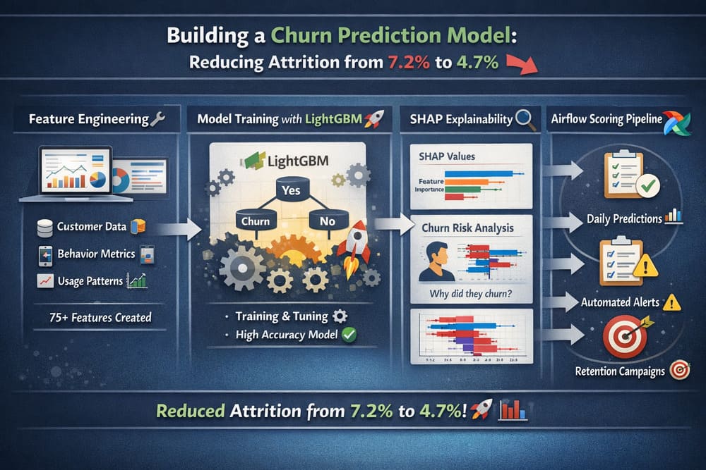
Consider a SaaS platform losing 7.2% of paying subscribers every month - nearly half its customer base a year. The hypothesis behind a churn model is that most of that churn is predictable weeks ahead, and that flagging at-risk customers early gives a retention team time to intervene. In one production deployment built on that premise, monthly churn dropped from 7.2% to 4.7% over three months - a 34% reduction. What follows is the full technical shape of that system: what worked, what didn't, and the code that matters.

Defining churn is harder than it looks

The first challenge is definitional, not technical. Churn means different things by business model: for monthly SaaS it's a subscription going from active to canceled or expired; for annual contracts it's failing to renew, which you must predict months ahead; for freemium it's dropping below a usage threshold or going inactive for N days, where the threshold is inherently arbitrary. For monthly billing, a workable definition is a customer whose status changes from "active" to "canceled" or "expired" within the next 30 days - 30 days gives the retention team enough runway for an email sequence, a CSM call, or a targeted walkthrough.

-- Churn label as a dbt model, materialized as a table
WITH subscription_changes AS (
    SELECT customer_id, status, changed_at,
           LAG(status) OVER (PARTITION BY customer_id ORDER BY changed_at) AS prev_status
    FROM subscription_events
    WHERE changed_at BETWEEN '2025-01-01' AND '2026-01-15'
),
churn_events AS (
    SELECT customer_id, changed_at AS churn_date
    FROM subscription_changes
    WHERE prev_status = 'active' AND status IN ('canceled', 'expired')
)
SELECT c.customer_id,
       CASE WHEN ce.customer_id IS NOT NULL THEN 1 ELSE 0 END AS churned
FROM customers c
LEFT JOIN churn_events ce ON c.customer_id = ce.customer_id
   AND ce.churn_date BETWEEN '2026-01-15' AND '2026-02-14'
WHERE c.subscription_status = 'active' AND c.subscription_start_date <= '2026-01-15';

The label-leakage trap: a tempting feature like "last payment date" is poison. If a monthly-billing customer's last payment was 28 days ago, they've almost certainly churned already - the model would be detecting the event, not predicting it. Every feature has to be audited so it contains only information available before the prediction window.

Features that actually predict churn

Of more than 60 features tested, the ones that survived fall into three categories. Product-usage features - windowed login counts, active days, and per-action counts plus trend ratios - carried the most signal:

def build_usage_features(events_df, prediction_date, customer_ids):
    features = pd.DataFrame({"customer_id": customer_ids})
    for window_days, suffix in [(7, "7d"), (14, "14d"), (30, "30d"), (90, "90d")]:
        cutoff = prediction_date - timedelta(days=window_days)
        win = events_df[(events_df.timestamp >= cutoff) & (events_df.timestamp <= prediction_date)]
        logins = win[win.event_type == "login"].groupby("customer_id").size() \
                    .reset_index(name=f"logins_{suffix}")
        features = features.merge(logins, on="customer_id", how="left")
        win = win.assign(date=win.timestamp.dt.date)
        active = win.groupby("customer_id").date.nunique().reset_index(name=f"active_days_{suffix}")
        features = features.merge(active, on="customer_id", how="left")
        for action in ["create_report", "invite_user", "export_data", "api_call"]:
            cnt = win[win.event_type == action].groupby("customer_id").size() \
                    .reset_index(name=f"{action}_{suffix}")
            features = features.merge(cnt, on="customer_id", how="left")
    features = features.fillna(0)
    # momentum: recent activity vs. the longer baseline
    features["active_days_trend"] = (features.active_days_7d / 7) / \
                                    (features.active_days_30d / 30).clip(lower=0.01)
    return features

Support and billing features add more - aggregated over 90 days, the counts of open tickets, negative-sentiment tickets, escalations, failed payments, downgrades, and upgrades. Account features (plan level, company-size bucket, account age) round it out as segmentation signals. The single most predictive feature was none of the obvious ones: it was active_days_trend, the ratio of active days in the last 7 days to the last 30. A customer active 20 of 30 days last month but only 1 of the last 7 is in serious trouble - and raw counts miss it, because 15 logins in 30 days looks healthy even when the last week is empty.

Handling class imbalance

With roughly 7% of customers churning in any 30-day window, a naive model drifts toward always predicting "no churn." Three approaches were compared with 5-fold stratified CV:

# 1) class weights
xgb_weighted = xgb.XGBClassifier(
    scale_pos_weight=(y_train == 0).sum() / (y_train == 1).sum(),
    n_estimators=500, max_depth=6, learning_rate=0.05, eval_metric="auc")
# 2) SMOTE oversampling to a 30% minority ratio
X_res, y_res = SMOTE(sampling_strategy=0.3, random_state=42).fit_resample(X_train, y_train)
# 3) LightGBM is_unbalance
lgb_model = lgb.LGBMClassifier(n_estimators=500, max_depth=6,
                               learning_rate=0.05, is_unbalance=True, verbose=-1)

# Results:
#   XGBoost + class_weight:  AUC = 0.856 (+/- 0.012)
#   XGBoost + SMOTE:         AUC = 0.861 (+/- 0.015)
#   LightGBM + is_unbalance: AUC = 0.872 (+/- 0.010)

LightGBM with is_unbalance=True won, but only by 1-2 AUC points. The honest takeaway is that the technique barely mattered next to feature engineering - good features handle moderate imbalance reasonably well regardless of the rebalancing method.

Training and choosing a threshold

The final model was a LightGBM classifier tuned with randomized search over depth, leaves, learning rate, subsampling, and regularization, scored on held-out AUC and average precision. The threshold is where business context dominates - it trades catching at-risk customers (recall) against not flooding the retention team with false alarms (precision):

precision, recall, thresholds = precision_recall_curve(y_test, y_probs)
# Threshold | Precision | Recall | Flagged | True churners caught
#   0.20    |   0.445   | 0.712  |   455   | 202
#   0.25    |   0.558   | 0.624  |   318   | 177
#   0.30    |   0.651   | 0.531  |   232   | 151
#   0.50    |   0.841   | 0.258  |    87   |  73

The chosen operating point was 0.25 - precision 0.558, recall 0.624. In plain terms: about 318 customers flagged per run, ~56% of whom will actually churn, catching 62% of all churners. The retention team could handle 300-400 outreach actions a week, so that was the right point. Final reported metrics: AUC-ROC 0.872, average precision 0.491 (against a 0.07 baseline).

Explaining each score with SHAP

A churn score without explanation is nearly useless to a retention team. "Customer X has 73% churn risk" is interesting; "73% because their logins dropped 80% this week and they have two unresolved tickets" is actionable. A tree SHAP explainer gives both global importance and per-customer reasons:

explainer = shap.TreeExplainer(best_model)
shap_values = explainer.shap_values(X_test)

# Global importance (mean |SHAP|), top features:
#   1. active_days_trend          (0.0834)
#   2. login_trend                (0.0721)
#   3. logins_7d                  (0.0645)
#   5. negative_sentiment_tickets (0.0498)
#   6. failed_payments_90d        (0.0456)

def explain(idx):
    contributions = sorted(zip(feature_names, shap_values[idx], X_test[idx]),
                           key=lambda x: abs(x[1]), reverse=True)
    risk = [{"feature": f, "value": round(float(v), 2),
             "impact": round(float(s), 4),
             "direction": "increases risk" if s > 0 else "decreases risk"}
            for f, s, v in contributions[:5]]
    return {"churn_probability": round(float(y_probs[idx]), 4), "factors": risk}

The per-customer explanation became the most valued part of the whole system - the retention team could see exactly why each customer was flagged and tailor the outreach.

Daily scoring pipeline

The model scores every active customer each morning before the retention team starts. The shape is a five-task Airflow DAG: extract features, score, write to the warehouse, push high-risk customers to the CRM, and post a Slack summary.

dag = DAG("churn_scoring_daily", schedule_interval="0 6 * * *",
          start_date=datetime(2026, 1, 1), catchup=False, tags=["ml", "churn"])

def extract_features(**ctx):
    d = pd.Timestamp(ctx["ds"]); conn = get_warehouse_connection()
    customers = pd.read_sql("SELECT * FROM customers WHERE subscription_status='active'", conn)
    # pull 90d of events / tickets / billing, then build the three feature blocks
    feats = (build_usage_features(events, d, ids)
             .merge(build_support_features(tickets, billing, d, ids), on="customer_id", how="left")
             .merge(build_account_features(customers, d), on="customer_id", how="left").fillna(0))
    feats.to_parquet(f"/tmp/churn_features_{ctx['ds']}.parquet")

def score_customers(**ctx):
    art = joblib.load("/models/churn/latest/model.joblib")
    feats = pd.read_parquet(ctx["ti"].xcom_pull(key="features_path"))
    probs = art["model"].predict_proba(feats[art["feature_columns"]].values)[:, 1]
    scores = feats[["customer_id"]].assign(
        churn_probability=probs,
        risk_level=pd.cut(probs, [0, 0.15, 0.25, 0.50, 1.0],
                          labels=["low", "medium", "high", "critical"]))
    scores.to_parquet(f"/tmp/churn_scores_{ctx['ds']}.parquet")

# write_to_warehouse upserts customer_health; push_to_crm syncs high/critical to HubSpot;
# send_slack_summary posts the daily risk breakdown.
extract >> score >> [warehouse, crm] >> slack

A companion dashboard reads the daily scores and shows three views: revenue at risk (total MRR in the high/critical buckets - "$47K MRR at critical risk this week" gets executive attention far faster than "127 customers might churn"), individual customer cards (score, 30-day trend, SHAP risk factors, a button to create a retention task), and intervention outcomes (which flagged customers got outreach and whether they stayed - the feedback loop for model improvement).

Results after three months

Metric	Before	After (3 months)	Change
Monthly churn rate	7.2%	4.7%	-34%
Revenue saved (est.)	-	$124K MRR	-
Retention team save rate	12% (random outreach)	31% (model-targeted)	+158%
Customers scored daily	0	8,400	-

The 34% reduction comes with an important caveat: the model alone didn't reduce churn. It identified at-risk customers; the retention team's outreach - personalized emails, CSM calls, walkthroughs, strategic discounts - saved them. The model was the targeting mechanism, not the intervention.

What didn't work

• Deep learning (LSTM on event sequences). Two weeks of work for 1.5 AUC points, at 20 minutes to score all customers instead of 30 seconds. Not worth it.
• NPS as a feature. Quarterly surveys were too stale to capture real-time sentiment shifts and added almost no predictive power.
• Automated email triggers. Auto-sending "we miss you" emails on a threshold annoyed happy customers. Switching to human-in-the-loop - model flags, human decides - fixed it.

Monitoring and retraining

An unmonitored churn model degrades. Three checks run weekly: prediction-distribution drift (alert if the mean score shifts more than ~15% from baseline), realized performance (compare 30-day-lagged actual churn against predicted, alert if realized AUC falls more than 0.05 below training), and feature-distribution shifts on the top features. Retraining happens monthly on the last six months of data, automated but gated on a human approval step - the new model must beat the current one on a held-out validation period before going live. This matters: in one stretch, AUC fell from 0.87 to 0.81 over two months after a product launch changed usage patterns, and only monitoring caught it.

Lessons

• Spend ~70% of the time on features, not models. The best AUC gain came from the activity-trend ratio, not from switching algorithms.
• Set the threshold with the business. The right cutoff depends on the cost of intervention versus the value of a saved customer - a business decision, not a statistical one.
• Explainability isn't optional. Without SHAP, the retention team ignored the model; with it, adoption was immediate.
• Monitor continuously. Usage patterns shift; monthly retraining catches the drift that silent models miss.
• The model is the easy part. The hard part is the operational workflow - scoring pipeline, CRM integration, retention processes, and feedback loops.

Feature category	Impact	Notes
Active days (incl. trend)	Highest	Single most important category - momentum beats levels
Login activity	High	Trend ratio more predictive than raw counts
Feature usage	High	Breadth (how many features) beat depth (how much of one)
Support tickets	Medium-high	Negative sentiment was key; total count alone was weak
Billing events	Medium	Failed payments strong; upgrades protective
Account attributes	Low-medium	Good for segmentation, weak standalone
NPS / survey	Low	Too infrequent to capture real-time risk

Churn prediction isn't a solved problem - every business has unique signals and unique retention levers. But the framework holds: start with features that capture behavioral momentum (trends, not just levels), build the scoring pipeline early even before the model is perfect, and invest most of the effort in the operational workflow that turns predictions into actions.