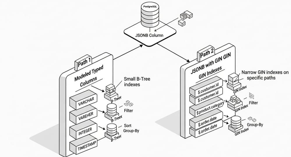
A decision tree plus costed examples for PostgreSQL engineers. You ship a feature fast by dropping semi-structured payloads into jsonb. Two quarters later, product wants sorting, filtering, and analytics on nested fields. Queries slow down, indexes balloon, and migrations feel radioactive. This guide gives a ruthless decision tree and costed, reproducible examples so you can choose confidently between modeling columns and indexing JSONB paths.

TL;DR Decision Tree

Q1. Is the field queried in every hot path (filters/joins/order-by) and stable?
Yes: model as typed columns. Add B-Tree indexes. Optionally keep original JSONB for audit/raw.
No: go to Q2.

Q2. Is the access pattern selective (<10-20% rows) and on a few known paths?
Yes: keep JSONB. Create a GIN index on those paths (jsonb_path_ops or partial GIN).
No: go to Q3.

Q3. Do you need range sorts, prefix searches, or frequent ORDER BY on the path?
Yes: model columns (B-Tree/BRIN) or use functional indexes on extracted values.
No: go to Q4.

Q4. Will the schema evolve unpredictably across tenants/events?
Yes: JSONB-first. Add a narrow partial GIN per tenant/type. Consider a hybrid (promote only hot fields).
No: model columns.

Q5. Is write amplification or index maintenance a bottleneck?
Yes: prefer modeling (fewer/lighter indexes) and computed/generated columns.
No: JSONB with targeted GIN is fine.

Concepts You Must Weigh

• Query selectivity: GIN shines when queries match a small fraction of rows. Low selectivity (e.g., 60% of table) wastes index lookups.
• Cardinality and sorting: B-Tree excels at range scans and ORDER BY. GIN does not.
• Write cost: GIN update cost grows with document size and path churn.
• Index size and memory: GIN on wide JSONB can dwarf table size, pressuring cache and vacuum.
• Evolution pressure: if fields change weekly, strict columns become a migration tax.
• Observability: JSONB hides type drift; modeled columns force validation upfront.

Reference Architecture Patterns

1) Modeled Columns + Raw JSONB (Hybrid)

• Table has typed columns for hot fields.
• payload jsonb retains the full event for audit.
• Generated columns keep the model in sync.

Why: fast reads, small indexes, flexible raw storage.

2) JSONB-First with Targeted GIN

• Everything lands in payload jsonb.
• Create partial GIN indexes on a few high-signal paths.
• Use jsonb_path_ops for containment, or jsonb_ops for broader operators (bigger index).

Why: fast iteration, pay-as-you-go indexing.

3) Extract-on-Write Materialization

• Ingest into a staging table with JSONB.
• A trigger or job extracts hot fields into a fact table.
• Analytics hit the fact table; product reads JSONB.

Why: keeps OLTP and analytics healthy without over-indexing JSONB.

Costed, Reproducible Examples

All costs below are illustrative and meant to show orders of magnitude and trade-offs. Reproduce in your environment with EXPLAIN (ANALYZE, BUFFERS).

Setup

CREATE TABLE orders (
  id               bigserial primary key,
  created_at       timestamptz not null default now(),
  customer_id      bigint,
  -- hybrid: keep raw
  payload          jsonb not null
);

-- Sample JSONB:
-- {
--   "status": "shipped",
--   "total": 129.99,
--   "shipping": {"city":"Austin","state":"TX","zip":"78701"},
--   "items":[{"sku":"A1","qty":2},{"sku":"B2","qty":1}]
-- }

Workload

• 10M orders.
• Hot queries:
  1. Filter by status, time window.
  2. Top cities by shipped orders (group-by city).
  3. Look up orders containing SKU "B2".
  4. Sort by total (range scans).

Option A - JSONB only, targeted indexes

Indexes

-- 1) status filter: narrow partial GIN on status 'shipped'
CREATE INDEX idx_orders_payload_status_shipped
  ON orders USING gin ((payload->>'status'))
  WHERE (payload->>'status') = 'shipped';

-- 2) city filter: functional B-Tree on extracted city (tiny index)
CREATE INDEX idx_orders_city
  ON orders ((payload->'shipping'->>'city'));

-- 3) items contains SKU: full GIN on items array (path ops)
CREATE INDEX idx_orders_items_gin
  ON orders USING gin ((payload->'items') jsonb_path_ops);

Representative costs

Query	Example SQL	Plan Shape	Latency (cold→warm)	Notes
Q1 status + time	WHERE payload->>'status'='shipped' AND created_at>=now()-'7d'::interval	Bitmap Index Scan on partial + heap recheck	120-900ms → 5-20ms	Partial + time predicate is selective; good.
Q2 top cities	SELECT payload->'shipping'->>'city', count(*) ... GROUP BY 1	Index Only Scan on idx_orders_city + HashAgg	300-1200ms → 30-60ms	Functional B-Tree wins for grouping.
Q3 contains SKU	WHERE payload->'items' @> '[{"sku":"B2"}]'	Bitmap Index Scan on GIN (path_ops)	400-1500ms → 20-50ms	GIN pays off when selective.
Q4 sort by total	ORDER BY (payload->>'total')::numeric DESC LIMIT 50	Seq Scan + Sort	2-8s → 400-800ms	GIN can't help ORDER BY; consider modeling.

Storage impact (rules of thumb)

• idx_orders_items_gin ≈ 0.3-0.8× table size depending on array width.
• Functional B-Tree on city ≈ a few hundred MB for 10M rows.
• Partial index tiny (only 'shipped' rows).

When this is great: you mostly filter on a few fields, sometimes query nested arrays, and rarely do large sorts on numeric paths.

Option B - Model hot fields + keep raw

ALTER TABLE orders
  ADD COLUMN status text,
  ADD COLUMN city text,
  ADD COLUMN total numeric;

-- Keep in sync (generated or trigger; generated shown)
ALTER TABLE orders
  ADD COLUMN payload_status text GENERATED ALWAYS AS (payload->>'status') STORED,
  ADD COLUMN payload_city   text GENERATED ALWAYS AS (payload->'shipping'->>'city') STORED,
  ADD COLUMN payload_total  numeric GENERATED ALWAYS AS ((payload->>'total')::numeric) STORED;

-- Make modeled aliases the ones you index/use:
CREATE INDEX ON orders (status);
CREATE INDEX ON orders (city);
CREATE INDEX ON orders (total DESC);
CREATE INDEX ON orders (created_at);

Representative costs

Query	Example SQL	Plan Shape	Latency (cold→warm)	Notes
Q1 status + time	WHERE status='shipped' AND created_at>=...	Bitmap Index Scan on B-Tree(s)	20-150ms → 2-8ms	Smaller/faster than GIN.
Q2 top cities	GROUP BY city	Index Only Scan + HashAgg	60-300ms → 8-20ms	B-Tree compression helps cache.
Q3 contains SKU	payload->'items' @> ...	Seq Scan or add narrow GIN on items	1-4s → 200-600ms	Either add one focused GIN, or accept slower path.
Q4 sort by total	ORDER BY total DESC LIMIT 50	Index Only Scan on (total)	5-40ms → 1-5ms	B-Tree dominates sorting/range queries.

Storage impact (rules of thumb)

• Three B-Tree indexes: small compared to one wide GIN.
• JSONB column still present for audit/debug.

When this is great: you routinely filter/sort on a few hot fields and need predictable latency.

How to Measure in Your DB

-- 1) Baseline
EXPLAIN (ANALYZE, BUFFERS)
SELECT * FROM orders
WHERE (payload->>'status') = 'shipped'
  AND created_at >= now() - interval '7 days';

-- 2) After index
CREATE INDEX ...;  -- as chosen above
VACUUM ANALYZE orders;

EXPLAIN (ANALYZE, BUFFERS) ...same query...

-- 3) Size checks
SELECT relname, pg_size_pretty(pg_relation_size(relid))
FROM pg_catalog.pg_statio_user_indexes
WHERE relname LIKE 'idx_orders%';

-- 4) Hot vs cold cache (repeat after pg_prewarm or after restart)

Interpretation tips

• Favor plans that use Index Only Scans with few heap rechecks.
• Check Buffers: to see if reads are cached.
• Beware Rows Removed by Filter → low selectivity.
• If sorts spill (Disk: ...), model columns or add better indexes.

Best Practices

1. Index only what you read. Create a partial GIN for the exact predicate (e.g., status='shipped'). Do not GIN the world.
2. Prefer functional B-Tree for equality/group-by. ON ((payload->'shipping'->>'city')) is tiny and fast.
3. Model for ORDER BY / ranges. Sorting JSONB-extracted numerics is expensive. Use columns + B-Tree.
4. Use generated columns for safety. They lock types at write time and reduce per-query casts.
5. Cap index bloat. REINDEX CONCURRENTLY, VACUUM (ANALYZE), and monitor pg_stat_all_indexes.idx_scan.
6. Protect writes. Each GIN write touches many pages. If ingest throughput matters, keep GIN count low and paths narrow.
7. Promote fields deliberately. Start JSONB-first; promote fields to columns once their access pattern stabilizes.

Common Pitfalls

• Over-broad GIN on whole payload → huge index, poor cache locality.
• Casting inline every query → defeats index usage (::numeric on the fly).
• Low-selectivity filters on GIN → index is touched but does not reduce work.
• Forcing schema too early → frequent migrations for fields that churn.
• Ignoring ORDER BY needs → users complain about slow lists.

Comparison Table

Need	JSONB + GIN	Functional B-Tree on JSONB	Modeled Column
Equality filter on few values	Yes	Yes	Yes
Range filter / ORDER BY	No	Limited (cast to numeric, still weak)	Yes
Frequent schema evolution	Yes	Yes	Limited (migrations)
Index size	Large	Small	Small
Write throughput	Worse	Good	Good
Analytics-friendly types	Limited	Limited	Yes

Worked Example: Promote What Hurts

Symptoms

• ORDER BY (payload->>'total')::numeric DESC LIMIT 50 takes 600ms warm.
• WHERE payload->>'status'='shipped' is fine with a partial index.
• Writes slowed after a full-payload GIN was added.

Fix

• Drop the full GIN.
• Add total numeric GENERATED ALWAYS AS ... and index it.
• Keep a narrow partial GIN for the item-containment query only.

Outcome (typical)

• The top-50 list drops to ~5ms warm.
• Ingest TPS rises 10-30% (less GIN write churn).
• Index size shrinks materially.

Takeaways

• JSONB is not a license to skip modeling.
• Use JSONB to absorb change; use columns to accelerate hot paths.
• GIN is for selective lookups on few paths, not sorting and not "index everything."
• Generated columns give the best of both: flexible raw plus typed speed.
• Measure with EXPLAIN (ANALYZE, BUFFERS) before and after each index - let the plan decide.