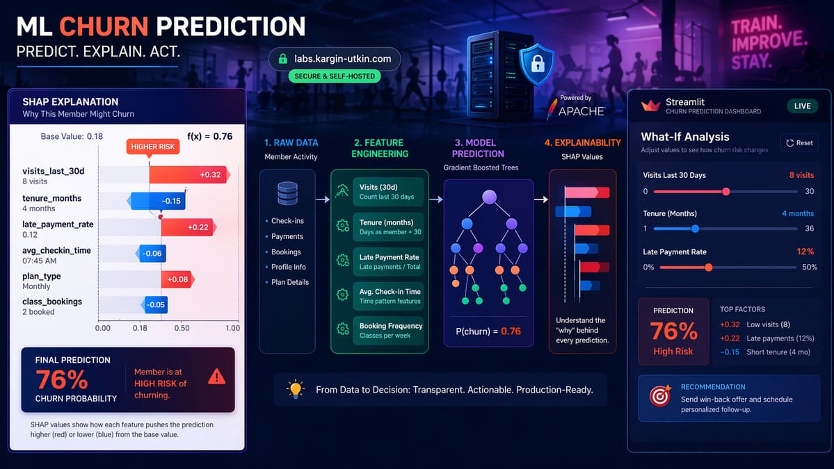
This is an end-to-end churn prediction system for fitness studio members - synthetic data generation, feature engineering, model training, SHAP explainability, and an interactive Streamlit demo deployed on self-hosted infrastructure, built in one focused session. The writeup covers the build, the lessons, and a live demo at labs.kargin-utkin.com/gym-churn.

The goal wasn't an expert-level paper on churn modeling. It was to rebuild the kind of system that runs in production at fitness and franchise chains, end-to-end, so every piece is understood by hand rather than conceptually.

The problem: member churn prediction

Every subscription business loses members. For a fitness chain - Orange Theory, Equinox, a boutique studio - identifying at-risk members before they cancel is worth millions. A retention call to someone about to quit can save an account. A call to someone who's already happy wastes budget.

So the model's job is: given a member's behavior - visit frequency, tenure, payment history, distance from studio, class variety - output two things:

1. A churn probability (will they cancel in the next 30 days?)
2. The reasons that probability is what it is (which behaviors pushed it up or down?)

The reasons matter more than the probability. A retention manager can't act on "this member has 73% churn risk." They need: "this member has dropped from 12 visits last month to 3, has two late payments, and lives 8 miles from their home studio." That's something you can pick up the phone about.

Why synthetic data

Real member data is never available outside the company that owns it - HIPAA-adjacent concerns, contractual restrictions, and privacy issues rule it out for a portfolio project. The standard workaround is synthetic data that mimics real patterns.

The generator produces 5,000 members with realistic behavioral correlations: declining visit frequency increases churn probability, longer tenure decreases it, late payments are a strong positive signal, friend referrals are a protective factor, morning visitors are stickier than afternoon-only ones. The churn label comes from a logistic probability function with noise - not random sampling - so a trained model has genuine signal to learn.

The important point: the model never sees the formula. It only sees features and labels. Whatever patterns it discovers, it discovers on its own. Swap the CSV for real OTF data tomorrow and nothing else in the pipeline changes.

The pipeline

Six stages, each in its own Python module:

src/
├── generate_data.py    # 5,000 synthetic members, realistic correlations
├── features.py         # 24 engineered features, stratified train/test split
├── train.py            # Logistic Regression baseline + XGBoost
├── explain.py          # SHAP: beeswarm, bar, dependence, waterfall
├── app.py              # Streamlit demo with 5 interactive tabs
└── ...

1. Feature engineering

Raw columns from the generator: age, gender, membership type, tenure, visit counts in 30/60/90-day windows, visit trend, days since last visit, percentage of morning visits, unique class types attended, late payments, distance in miles.

On top of those sit interaction features and ratios that capture domain-specific risk patterns:

• new_and_declining - binary flag for (tenure < 6 months) AND (visits declining > 20%). New members with falling engagement are the highest-risk segment.
• far_and_basic - distant + cheap plan = low commitment signal.
• visits_per_mile - a loyalty proxy: frequent visitors who travel far are highly invested.
• late_payment_rate - normalizes late payments by tenure so a 12-month member with 1 late payment isn't scored the same as a 1-month member with 1 late payment.
• visit_accel - second derivative of visits: is the decline accelerating?

24 features total after encoding. These take about 20 lines of pandas code and matter more than model choice. For tabular problems, feature engineering is where the wins are; model choice is a minor tweak at the end.

2. Training two models

This build trains both a Logistic Regression baseline and an XGBoost classifier. Why two?

Because every real-world ML project needs a baseline. If a gradient-boosted ensemble beats logistic regression by 2 points of AUC, that's a lot of complexity for very little gain. If it beats it by 10 points, the problem actually needs nonlinearity. The comparison is what tells the story.

Results on the held-out test set:

Metric	Logistic Regression	XGBoost
AUC-ROC	0.815	0.790
Precision (churners)	0.41	0.48
Recall (churners)	0.71	0.53
Accuracy	0.76	0.81

Logistic Regression wins on AUC and recall. XGBoost wins on precision and accuracy. The choice depends entirely on the business context. In a retention-outreach scenario where calling one extra happy member beats missing a real churner, recall matters more than precision, and LogReg is the better model here.

That trade-off doesn't show up on a Kaggle leaderboard. It only matters once you account for what happens after the prediction.

3. SHAP: the part that makes it usable

SHAP (SHapley Additive exPlanations) is the interpretability tool that turns any tree-based model into something you can explain to a non-technical stakeholder.

For each prediction, SHAP assigns each feature a value that represents how much that feature pushed the prediction up or down relative to the base rate. Sum all the SHAP values for a member and you get the total prediction. It's exact, not approximated.

Three things SHAP provides:

• Global feature importance - average absolute SHAP value per feature across all members. Tells you which features drive the model overall.
• Beeswarm plots - scatter of SHAP values per member, color-coded by feature value. Shows direction and spread: high visit counts push predictions down (green dots on the left), low visit counts push them up (red dots on the right).
• Waterfall plots - per-member breakdown. "This member is predicted 73% churn risk. +20% from low visits, +15% from late payments, -12% from long tenure, -5% from referral." That's the retention-manager-facing explanation.

Top churn drivers in this model, by mean |SHAP|: visits_last_30d (dominates), tenure_months, unique_class_types, visit_trend, late_payment_rate.

Visit frequency is always #1 in a fitness churn model - that part is well known. The more useful question is what else matters, and how the interactions between features change individual predictions. SHAP makes those interactions visible.

Self-hosted, not Streamlit Cloud

The demo lives at labs.kargin-utkin.com/gym-churn, running on a self-managed server behind Apache with a Let's Encrypt cert and WebSocket tunneling for live Streamlit updates.

Free services like Streamlit Community Cloud were avoided on purpose, for two reasons:

1. Data privacy. The app has an upload feature where users can score their own members. Sending real gym data through a third-party service is a non-starter. On self-hosted infrastructure, the claim holds: nothing is stored on disk, processed in memory only, never shared.
2. Positioning. This lab belongs to InnovaTek, an on-premise AI consultancy. The portfolio should demonstrate self-hosted ML directly, not depend on somebody else's free tier.

The architecture is simple: the Streamlit app runs as a systemd service bound to 127.0.0.1:8501. Apache reverse-proxies labs.kargin-utkin.com/gym-churn to that port, including WebSocket upgrade for live slider updates. Each future lab app gets its own port and systemd service - clean failure isolation, so one app crashing doesn't take others down.

The demo has 5 tabs

1. Overview - model metrics, churn probability distribution, table of the 20 highest-risk members.
2. Feature Importance - global SHAP plots.
3. Member Lookup - enter any member ID, see their predicted risk and the SHAP waterfall explaining it.
4. What-If Simulator - sliders to adjust member attributes and watch predictions update in real time.
5. Upload Your Data - CSV upload, returns a scored CSV with churn probability, risk level, and top 3 SHAP reasons per member. Processed in memory only.

The What-If tab is the most instructive. Move the "visits last 30d" slider from 15 down to 0 and the prediction jumps. Move late payments from 0 to 5 and it jumps again. This is how the model "thinks" made concrete.

What the build confirmed

A few things that stood out:

• Feature engineering > model choice. The interaction features (new_and_declining, far_and_basic) appeared in SHAP's top ranks - the model found them useful. Hand-crafted features that encode domain knowledge still beat "throw more data at a bigger model" for tabular problems.
• The baseline held up. Logistic Regression came out ahead on recall, which is what matters for this problem. A lot of real production ML is simpler than the literature implies.
• SHAP is the unlock. Without it, the output is just "a number came out of a machine." With it, it's "here are the three reasons." That difference is what lets a business actually use the model.
• Self-hosting is less work than it looks. Apache vhost + systemd + Let's Encrypt + DNS took a few hours total. Once the pattern is established, the next lab app is essentially copy-paste.

What's next

The roadmap:

• Validate on real public data - Kaggle has a fitness member churn dataset. Running the same pipeline on real data is the harder test.
• Hyperparameter tuning - currently using defaults; adding Optuna shows how far the gap between LogReg and XGBoost closes (or opens) with proper tuning.
• Time-series features - weekly cohort tracking, seasonality, multi-month trends. The current model treats each member as a snapshot; real systems track trajectories.
• More lab apps - next up is franchise demand forecasting (1-hour-ahead predictions per location, per product). Same infrastructure, different domain.

Links

Live demo: labs.kargin-utkin.com/gym-churn

Code: github.com/alexnews/labs.kargin-utkin.com