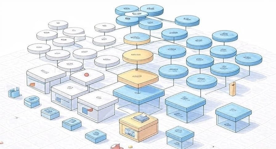
Schema design is the backbone of every data warehouse, and it's a balancing act between competing priorities: query performance, storage efficiency, maintenance complexity, data integrity, and how intuitive the model is for analysts. Those factors conflict - optimizing one usually costs another - which is why three patterns persist rather than one winning outright: normalized schemas, star schemas, and snowflake schemas. Each makes a different trade among those priorities.

Normalized schemas

Normalization organizes data to minimize redundancy and dependency by decomposing tables into smaller, related ones connected through foreign keys (the normal forms - 1NF removes repeating groups, 2NF removes partial dependencies, 3NF removes transitive dependencies, BCNF tightens 3NF). The result is many purpose-specific tables, referential integrity, minimal redundancy, and complex joins for comprehensive queries.

-- E-commerce normalized schema (excerpt)
CREATE TABLE customers (
    customer_id INT PRIMARY KEY,
    first_name VARCHAR(50), last_name VARCHAR(50),
    email VARCHAR(100), registration_date DATE
);
CREATE TABLE products (
    product_id INT PRIMARY KEY, product_name VARCHAR(100),
    category_id INT, price DECIMAL(10,2),
    FOREIGN KEY (category_id) REFERENCES categories(category_id)
);
CREATE TABLE orders (
    order_id INT PRIMARY KEY, customer_id INT, order_date DATE,
    total_amount DECIMAL(10,2),
    FOREIGN KEY (customer_id) REFERENCES customers(customer_id)
);
CREATE TABLE order_items (
    order_item_id INT PRIMARY KEY, order_id INT, product_id INT,
    quantity INT, unit_price DECIMAL(10,2),
    FOREIGN KEY (order_id) REFERENCES orders(order_id),
    FOREIGN KEY (product_id) REFERENCES products(product_id)
);

The strengths are data integrity (changes happen in one place), storage efficiency (no redundant data), and flexibility to add attributes without disrupting existing structure. The costs are query complexity (comprehensive analysis needs many joins), slower execution from those joins, and a model that's harder for business users to navigate. Normalized schemas fit OLTP systems, integrity-critical applications, frequent-update environments, and cases where storage cost dominates.

Star schema

The star schema is a dimensional pattern built for analytics: a central fact table holding quantitative measures and foreign keys, surrounded by denormalized dimension tables holding descriptive attributes for filtering and grouping.

-- Sales analytics star schema
CREATE TABLE fact_sales (
    sale_id INT PRIMARY KEY,
    customer_key INT, product_key INT, date_key INT, store_key INT,
    quantity_sold INT, unit_price DECIMAL(10,2),
    total_revenue DECIMAL(12,2), profit DECIMAL(12,2),
    FOREIGN KEY (customer_key) REFERENCES dim_customer(customer_key),
    FOREIGN KEY (product_key)  REFERENCES dim_product(product_key),
    FOREIGN KEY (date_key)     REFERENCES dim_date(date_key),
    FOREIGN KEY (store_key)    REFERENCES dim_store(store_key)
);
CREATE TABLE dim_customer (
    customer_key INT PRIMARY KEY, customer_id VARCHAR(20),
    customer_name VARCHAR(100), customer_segment VARCHAR(50),
    customer_region VARCHAR(50), customer_country VARCHAR(50)
);
CREATE TABLE dim_date (
    date_key INT PRIMARY KEY, full_date DATE, day_of_week VARCHAR(10),
    month_name VARCHAR(10), quarter VARCHAR(10), year INT,
    is_weekend BOOLEAN, is_holiday BOOLEAN
);  -- dim_product and dim_store follow the same denormalized shape

The denormalized dimensions give the star schema its advantages: simple joins and fast queries, an intuitive structure for business users, and a layout most BI tools are optimized for. The cost is storage overhead and redundancy from the denormalization, plus update complexity when dimensional data changes across many rows. Star schemas fit data warehouses, BI and reporting systems, OLAP workloads, and anything needing fast aggregation and filtering.

Snowflake schema

The snowflake schema extends the star by normalizing dimensions into multiple related tables, producing branching hierarchies - less redundancy than a star, but more joins.

-- Fact table is unchanged; dimensions are normalized
CREATE TABLE dim_customer (
    customer_key INT PRIMARY KEY, customer_id VARCHAR(20),
    customer_name VARCHAR(100), customer_segment_key INT, region_key INT,
    FOREIGN KEY (customer_segment_key) REFERENCES dim_customer_segment(segment_key),
    FOREIGN KEY (region_key) REFERENCES dim_geography(geography_key)
);
CREATE TABLE dim_customer_segment (
    segment_key INT PRIMARY KEY, segment_name VARCHAR(50), segment_description TEXT
);
CREATE TABLE dim_product_category (   -- self-referencing hierarchy
    category_key INT PRIMARY KEY, category_name VARCHAR(50), parent_category_key INT,
    FOREIGN KEY (parent_category_key) REFERENCES dim_product_category(category_key)
);
CREATE TABLE dim_geography (
    geography_key INT PRIMARY KEY, city VARCHAR(50), state VARCHAR(50),
    country VARCHAR(50), region VARCHAR(50), continent VARCHAR(50)
);

The advantages are storage efficiency, preserved referential integrity, natural representation of hierarchies, and easier modification of dimensional structures. The costs are more joins, slower queries, and more tables to manage. Snowflake schemas fit complex dimensional hierarchies, storage-constrained environments, integrity-sensitive systems, and dimensions that change frequently.

Performance optimization

Across all dimensional models, three levers do most of the work. Index the fact-table foreign keys and the dimension business keys (the snowflake schema needs extra indexes on the normalized dimension relationships). Partition fact tables by date so queries prune to the relevant ranges:

CREATE TABLE fact_sales_partitioned (...)
PARTITION BY RANGE (sale_date) (
    PARTITION p2023_q1 VALUES LESS THAN ('2023-04-01'),
    PARTITION p2023_q2 VALUES LESS THAN ('2023-07-01'),
    PARTITION p2023_q3 VALUES LESS THAN ('2023-10-01'),
    PARTITION p2023_q4 VALUES LESS THAN ('2024-01-01')
);

And materialize common aggregations so dashboards read pre-computed rollups instead of re-joining the fact table:

CREATE MATERIALIZED VIEW mv_monthly_sales AS
SELECT d.year, d.month_name, p.product_category, c.customer_segment,
       SUM(f.total_revenue) AS total_revenue,
       SUM(f.quantity_sold) AS total_quantity, COUNT(*) AS transaction_count
FROM fact_sales f
JOIN dim_date d     ON f.date_key = d.date_key
JOIN dim_product p  ON f.product_key = p.product_key
JOIN dim_customer c ON f.customer_key = c.customer_key
GROUP BY d.year, d.month_name, p.product_category, c.customer_segment;

Modern approaches

Beyond the three classics, Data Vault models around hub tables (business keys), link tables (relationships), and satellite tables (descriptive data) - strong for auditability and frequently-changing sources. dbt has become the standard way to build dimensional models, generating surrogate keys and materializing fact and dimension tables from staging models. And cloud warehouses change the optimization knobs: instead of classic indexes, Snowflake uses clustering keys (ALTER TABLE fact_sales CLUSTER BY (date_key, customer_key)) and BigQuery combines partitioning with clustering (PARTITION BY sale_date CLUSTER BY customer_key, product_key).

Choosing a schema

Choose a normalized schema for OLTP systems where data integrity is paramount, storage cost is critical, and updates are frequent. Choose a star schema for analytics warehouses where query performance is the top priority, business users need direct access, and BI tools are the primary interface. Choose a snowflake schema when complex hierarchical dimensions exist, storage efficiency matters but performance still counts, and dimensional structures change often. In practice the star schema is the default for analytics, with selective snowflaking of the dimensions that have genuine hierarchies - getting most of the star's query speed while taming the worst of its redundancy.