Data Modeling Concepts: Normalized, Star, and Snowflake Schemas – A Complete Guide for Data Professionals
Introduction
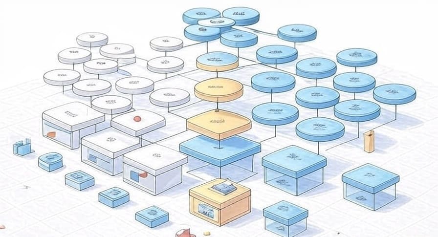
Data modeling forms the backbone of every successful data warehouse and analytics platform. Whether you’re designing a new data architecture or optimizing an existing one, understanding the fundamental schema design patterns is crucial for building scalable, performant, and maintainable data systems.
This article explores three essential data modeling approaches: Normalized schemas, Star schemas, and Snowflake schemas. We’ll examine their structures, advantages, trade-offs, and real-world applications to help you make informed architectural decisions for your data projects.
Who should read this? Data Engineers, Database Architects, Analytics Engineers, and Data Scientists working with data warehouses, business intelligence systems, or analytical databases.
What you’ll learn: The core principles of each schema type, when to use them, performance implications, and practical implementation strategies.
Understanding Data Schema Design Fundamentals
Before diving into specific schema types, it’s essential to understand the driving forces behind different data modeling approaches:
Query Performance: How quickly can users retrieve insights from the data?
Storage Efficiency: How much disk space does the schema consume?
Maintenance Complexity: How easy is it to modify and maintain the schema over time?
Data Integrity: How well does the schema prevent inconsistent or duplicate data?
User Experience: How intuitive is the schema for analysts and business users?
These factors often conflict with each other, making schema design a balancing act between competing priorities.
Normalized Schemas: The Foundation of Relational Design
What is Normalization?
Normalization is a database design technique that organizes data to minimize redundancy and dependency. The process involves decomposing tables into smaller, related tables and defining relationships between them through foreign keys.
Normal Forms Overview
First Normal Form (1NF): Eliminates repeating groups and ensures atomic values Second Normal Form (2NF): Removes partial dependencies on composite keys Third Normal Form (3NF): Eliminates transitive dependencies Boyce-Codd Normal Form (BCNF): A stricter version of 3NF
Structure and Characteristics
Normalized schemas typically feature:
- Multiple related tables with specific purposes
- Foreign key relationships maintaining referential integrity
- Minimal data redundancy
- Complex join operations for comprehensive queries
Example: E-commerce Normalized Schema
sql-- Customers table
CREATE TABLE customers (
    customer_id INT PRIMARY KEY,
    first_name VARCHAR(50),
    last_name VARCHAR(50),
    email VARCHAR(100),
    registration_date DATE
);

-- Products table
CREATE TABLE products (
    product_id INT PRIMARY KEY,
    product_name VARCHAR(100),
    category_id INT,
    price DECIMAL(10,2),
    FOREIGN KEY (category_id) REFERENCES categories(category_id)
);

-- Categories table
CREATE TABLE categories (
    category_id INT PRIMARY KEY,
    category_name VARCHAR(50),
    description TEXT
);

-- Orders table
CREATE TABLE orders (
    order_id INT PRIMARY KEY,
    customer_id INT,
    order_date DATE,
    total_amount DECIMAL(10,2),
    FOREIGN KEY (customer_id) REFERENCES customers(customer_id)
);

-- Order_items table
CREATE TABLE order_items (
    order_item_id INT PRIMARY KEY,
    order_id INT,
    product_id INT,
    quantity INT,
    unit_price DECIMAL(10,2),
    FOREIGN KEY (order_id) REFERENCES orders(order_id),
    FOREIGN KEY (product_id) REFERENCES products(product_id)
);
Advantages of Normalized Schemas
Data Integrity: Strong referential integrity prevents inconsistent data Storage Efficiency: Eliminates redundant data storage Update Efficiency: Changes need to be made in only one place Flexibility: Easy to add new attributes without affecting existing structure
Disadvantages of Normalized Schemas
Query Complexity: Complex joins required for comprehensive analysis Performance Impact: Multiple joins can slow down query execution Learning Curve: More difficult for business users to understand and navigate
When to Use Normalized Schemas
Normalized schemas excel in:
- OLTP (Online Transaction Processing) systems
- Applications requiring high data integrity
- Environments with frequent data updates
- Systems where storage cost is a primary concern
Star Schema: The Analytics Powerhouse
Understanding Star Schema Design
The Star schema is a dimensional modeling technique optimized for analytical queries and business intelligence. It resembles a star with a central fact table surrounded by dimension tables.
Core Components
Fact Table: Contains quantitative data (measures) and foreign keys to dimension tables Dimension Tables: Contain descriptive attributes used for filtering and grouping
Structure and Characteristics
Star schemas feature:
- Denormalized dimension tables
- Central fact table with foreign keys
- Simple join patterns
- Optimized for read-heavy analytical workloads
Example: Sales Analytics Star Schema
sql-- Fact table: Sales Facts
CREATE TABLE fact_sales (
    sale_id INT PRIMARY KEY,
    customer_key INT,
    product_key INT,
    date_key INT,
    store_key INT,
    quantity_sold INT,
    unit_price DECIMAL(10,2),
    total_revenue DECIMAL(12,2),
    cost_of_goods DECIMAL(12,2),
    profit DECIMAL(12,2),
    FOREIGN KEY (customer_key) REFERENCES dim_customer(customer_key),
    FOREIGN KEY (product_key) REFERENCES dim_product(product_key),
    FOREIGN KEY (date_key) REFERENCES dim_date(date_key),
    FOREIGN KEY (store_key) REFERENCES dim_store(store_key)
);

-- Dimension table: Customer
CREATE TABLE dim_customer (
    customer_key INT PRIMARY KEY,
    customer_id VARCHAR(20),
    customer_name VARCHAR(100),
    customer_segment VARCHAR(50),
    customer_region VARCHAR(50),
    customer_country VARCHAR(50),
    registration_date DATE,
    customer_lifetime_value DECIMAL(12,2)
);

-- Dimension table: Product
CREATE TABLE dim_product (
    product_key INT PRIMARY KEY,
    product_id VARCHAR(20),
    product_name VARCHAR(100),
    product_category VARCHAR(50),
    product_subcategory VARCHAR(50),
    brand VARCHAR(50),
    supplier VARCHAR(100),
    unit_cost DECIMAL(10,2)
);

-- Dimension table: Date
CREATE TABLE dim_date (
    date_key INT PRIMARY KEY,
    full_date DATE,
    day_of_week VARCHAR(10),
    day_of_month INT,
    week_of_year INT,
    month_name VARCHAR(10),
    quarter VARCHAR(10),
    year INT,
    is_weekend BOOLEAN,
    is_holiday BOOLEAN
);

-- Dimension table: Store
CREATE TABLE dim_store (
    store_key INT PRIMARY KEY,
    store_id VARCHAR(20),
    store_name VARCHAR(100),
    store_type VARCHAR(50),
    store_size VARCHAR(20),
    city VARCHAR(50),
    state VARCHAR(50),
    region VARCHAR(50),
    manager_name VARCHAR(100)
);
Advantages of Star Schema
Query Performance: Simple joins lead to faster query execution User-Friendly: Intuitive structure for business users and analysts BI Tool Optimization: Most BI tools are optimized for star schema patterns Aggregation Efficiency: Pre-calculated measures improve reporting speed
Disadvantages of Star Schema
Storage Overhead: Denormalized dimensions increase storage requirements Data Redundancy: Duplicate data across dimension tables Update Complexity: Changes to dimensional data require updates across multiple records
When to Use Star Schema
Star schemas are ideal for:
- Data warehouses and analytical databases
- Business intelligence and reporting systems
- OLAP (Online Analytical Processing) applications
- Scenarios requiring fast aggregation and filtering
Snowflake Schema: The Balanced Approach
Understanding Snowflake Schema Design
The Snowflake schema extends the Star schema by normalizing dimension tables into multiple related tables, creating a structure that resembles a snowflake with branching patterns.
Structure and Characteristics
Snowflake schemas combine:
- Normalized dimension tables
- Hierarchical relationships within dimensions
- Reduced data redundancy compared to Star schema
- More complex join patterns than Star schema
Example: Sales Analytics Snowflake Schema
sql-- Fact table remains the same as Star schema
CREATE TABLE fact_sales (
    sale_id INT PRIMARY KEY,
    customer_key INT,
    product_key INT,
    date_key INT,
    store_key INT,
    quantity_sold INT,
    unit_price DECIMAL(10,2),
    total_revenue DECIMAL(12,2),
    FOREIGN KEY (customer_key) REFERENCES dim_customer(customer_key),
    FOREIGN KEY (product_key) REFERENCES dim_product(product_key),
    FOREIGN KEY (date_key) REFERENCES dim_date(date_key),
    FOREIGN KEY (store_key) REFERENCES dim_store(store_key)
);

-- Normalized Customer dimension
CREATE TABLE dim_customer (
    customer_key INT PRIMARY KEY,
    customer_id VARCHAR(20),
    customer_name VARCHAR(100),
    customer_segment_key INT,
    region_key INT,
    registration_date DATE,
    FOREIGN KEY (customer_segment_key) REFERENCES dim_customer_segment(segment_key),
    FOREIGN KEY (region_key) REFERENCES dim_geography(geography_key)
);

CREATE TABLE dim_customer_segment (
    segment_key INT PRIMARY KEY,
    segment_name VARCHAR(50),
    segment_description TEXT
);

-- Normalized Product dimension
CREATE TABLE dim_product (
    product_key INT PRIMARY KEY,
    product_id VARCHAR(20),
    product_name VARCHAR(100),
    category_key INT,
    brand_key INT,
    supplier_key INT,
    unit_cost DECIMAL(10,2),
    FOREIGN KEY (category_key) REFERENCES dim_product_category(category_key),
    FOREIGN KEY (brand_key) REFERENCES dim_brand(brand_key),
    FOREIGN KEY (supplier_key) REFERENCES dim_supplier(supplier_key)
);

CREATE TABLE dim_product_category (
    category_key INT PRIMARY KEY,
    category_name VARCHAR(50),
    parent_category_key INT,
    FOREIGN KEY (parent_category_key) REFERENCES dim_product_category(category_key)
);

CREATE TABLE dim_brand (
    brand_key INT PRIMARY KEY,
    brand_name VARCHAR(50),
    brand_country VARCHAR(50)
);

-- Normalized Geography dimension
CREATE TABLE dim_geography (
    geography_key INT PRIMARY KEY,
    city VARCHAR(50),
    state VARCHAR(50),
    country VARCHAR(50),
    region VARCHAR(50),
    continent VARCHAR(50)
);
Advantages of Snowflake Schema
Storage Efficiency: Reduced redundancy compared to Star schema Data Integrity: Normalized structure maintains referential integrity Hierarchical Modeling: Natural representation of hierarchical relationships Maintenance Flexibility: Easier to modify dimensional hierarchies
Disadvantages of Snowflake Schema
Query Complexity: More joins required for comprehensive analysis Performance Impact: Additional joins can slow query execution Increased Complexity: More tables to manage and understand
When to Use Snowflake Schema
Snowflake schemas work well for:
- Complex dimensional hierarchies
- Storage-constrained environments
- Systems requiring strong referential integrity
- Scenarios with frequently changing dimensional structures
Performance Considerations and Optimization Strategies
Indexing Strategies
Star Schema Indexing:
sql-- Create indexes on fact table foreign keys
CREATE INDEX idx_fact_sales_customer ON fact_sales(customer_key);
CREATE INDEX idx_fact_sales_product ON fact_sales(product_key);
CREATE INDEX idx_fact_sales_date ON fact_sales(date_key);

-- Create indexes on dimension table business keys
CREATE INDEX idx_dim_customer_id ON dim_customer(customer_id);
CREATE INDEX idx_dim_product_id ON dim_product(product_id);
Snowflake Schema Indexing:
sql-- Additional indexes for normalized dimension relationships
CREATE INDEX idx_customer_segment ON dim_customer(customer_segment_key);
CREATE INDEX idx_product_category ON dim_product(category_key);
CREATE INDEX idx_geography_region ON dim_geography(region);
Partitioning Strategies
sql-- Date-based partitioning for fact tables
CREATE TABLE fact_sales_partitioned (
    sale_id INT,
    customer_key INT,
    product_key INT,
    date_key INT,
    sale_date DATE,
    quantity_sold INT,
    total_revenue DECIMAL(12,2)
)
PARTITION BY RANGE (sale_date) (
    PARTITION p2023_q1 VALUES LESS THAN ('2023-04-01'),
    PARTITION p2023_q2 VALUES LESS THAN ('2023-07-01'),
    PARTITION p2023_q3 VALUES LESS THAN ('2023-10-01'),
    PARTITION p2023_q4 VALUES LESS THAN ('2024-01-01')
);
Materialized Views and Aggregations
sql-- Create materialized view for common aggregations
CREATE MATERIALIZED VIEW mv_monthly_sales AS
SELECT
    d.year,
    d.month_name,
    p.product_category,
    c.customer_segment,
    SUM(f.total_revenue) as total_revenue,
    SUM(f.quantity_sold) as total_quantity,
    COUNT(*) as transaction_count
FROM fact_sales f
JOIN dim_date d ON f.date_key = d.date_key
JOIN dim_product p ON f.product_key = p.product_key
JOIN dim_customer c ON f.customer_key = c.customer_key
GROUP BY d.year, d.month_name, p.product_category, c.customer_segment;
Modern Data Modeling Approaches
Data Vault Modeling
Data Vault is an alternative approach focusing on:
- Hub tables (business keys)
- Link tables (relationships)
- Satellite tables (descriptive data)
Dimensional Modeling with dbt
sql-- dbt model for star schema fact table
{{ config(materialized='table') }}

SELECT
    s.sale_id,
    {{ dbt_utils.surrogate_key(['c.customer_id']) }} as customer_key,
    {{ dbt_utils.surrogate_key(['p.product_id']) }} as product_key,
    {{ dbt_utils.surrogate_key(['s.sale_date']) }} as date_key,
    s.quantity_sold,
    s.unit_price,
    s.total_revenue
FROM {{ ref('stg_sales') }} s
LEFT JOIN {{ ref('dim_customer') }} c ON s.customer_id = c.customer_id
LEFT JOIN {{ ref('dim_product') }} p ON s.product_id = p.product_id
Cloud Data Warehouse Considerations
Snowflake-Specific Optimizations:
sql-- Clustering keys for better performance
ALTER TABLE fact_sales CLUSTER BY (date_key, customer_key);

-- Automatic clustering
ALTER TABLE fact_sales SET CLUSTER BY (date_key);
BigQuery Partitioning and Clustering:
sqlCREATE TABLE `project.dataset.fact_sales`
(
  sale_id INT64,
  customer_key INT64,
  product_key INT64,
  sale_date DATE,
  total_revenue NUMERIC
)
PARTITION BY sale_date
CLUSTER BY customer_key, product_key;
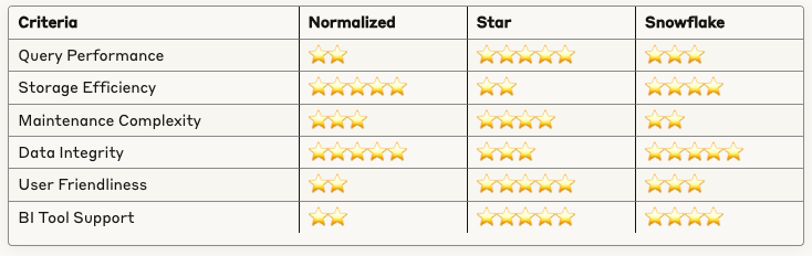
Schema Selection Decision Framework
Evaluation Criteria Matrix
Decision Guidelines
Choose Normalized Schema when:
- Building OLTP systems
- Data integrity is paramount
- Storage costs are critical
- Update frequency is high
Choose Star Schema when:
- Building data warehouses for analytics
- Query performance is top priority
- Business users need direct access
- BI tools are primary interface
Choose Snowflake Schema when:
- Complex hierarchical dimensions exist
- Storage efficiency matters but performance is still important
- Dimensional structures change frequently
- Hybrid OLTP/OLAP requirements exist
Implementation Best Practices
Design Phase Best Practices
- Understand Your Use Case: Clearly define whether you’re building for transactions or analytics
- Know Your Users: Consider the technical expertise of end users
- Plan for Scale: Design with future data volume growth in mind
- Consider Tool Ecosystem: Ensure compatibility with existing BI and analytics tools
Development Best Practices
sql-- Use consistent naming conventions
-- Example: Fact tables prefix 'fact_', dimension tables prefix 'dim_'

-- Implement proper constraints
ALTER TABLE fact_sales
ADD CONSTRAINT fk_sales_customer
FOREIGN KEY (customer_key) REFERENCES dim_customer(customer_key);

-- Create comprehensive documentation
COMMENT ON TABLE fact_sales IS 'Daily sales transactions with associated dimensions';
COMMENT ON COLUMN fact_sales.total_revenue IS 'Revenue in USD, including taxes';
Maintenance Best Practices
- Monitor Query Performance: Regularly review slow-running queries
- Update Statistics: Keep database statistics current for optimal query plans
- Archive Historical Data: Implement data retention policies
- Version Control: Track schema changes using database migration tools
Real-World Case Studies
Case Study 1: E-commerce Analytics Platform
Challenge: Global e-commerce company needed to support both operational reporting and advanced analytics across multiple business units.
Solution: Implemented a hybrid approach:
- Normalized schema for operational systems
- Star schema for executive dashboards
- Snowflake schema for detailed product analytics
Results: 40% improvement in dashboard load times, 60% reduction in storage costs for detailed analytics.
Case Study 2: Financial Services Data Warehouse
Challenge: Regional bank required regulatory reporting, risk analysis, and customer analytics from the same data platform.
Solution: Multi-layered architecture:
- Normalized staging layer for data quality
- Star schema marts for different business domains
- Specialized snowflake schemas for complex regulatory hierarchies
Results: Reduced time-to-insight from weeks to hours, improved regulatory compliance reporting accuracy.
Emerging Trends and Future Considerations
Modern Data Stack Integration
Contemporary data stacks often combine multiple schema approaches:
- ELT Pipelines: Raw data to normalized staging to dimensional marts
- Data Lakehouse: Schema-on-read capabilities supporting multiple modeling approaches
- Real-time Analytics: Stream processing with star schema for immediate insights
Cloud-Native Considerations
Modern cloud data platforms offer new capabilities:
- Automatic Optimization: Query engines that adapt to different schema patterns
- Elastic Scaling: Separate compute and storage for cost optimization
- Serverless Analytics: Reduced infrastructure management overhead
Key Takeaways and Recommendations
Essential Insights
- No One-Size-Fits-All: Each schema type serves specific use cases and requirements
- Performance vs. Flexibility: There’s always a trade-off between query performance and schema flexibility
- Evolution is Normal: Most organizations use multiple schema types across different systems
- Tool Integration Matters: Consider your analytics tool ecosystem when choosing schema patterns
Actionable Recommendations
For Data Engineers:
- Master all three schema types to make informed architectural decisions
- Implement automated testing for schema changes
- Monitor query performance across different schema patterns
- Document design decisions and trade-offs for future reference
For Data Architects:
- Develop organizational standards for schema selection criteria
- Create reusable dimensional models for common business concepts
- Plan for schema evolution and versioning strategies
- Consider data governance implications of each approach
For Analytics Teams:
- Understand the implications of different schema types on query performance
- Collaborate with engineering teams on optimal schema design
- Provide feedback on user experience across different schema patterns
- Advocate for schemas that support self-service analytics
Next Steps
- Assess Current State: Evaluate your existing data models against these patterns
- Define Requirements: Clearly articulate performance, usability, and maintenance needs
- Prototype and Test: Build small-scale implementations to validate design decisions
- Implement Gradually: Migrate to new schema patterns incrementally
- Monitor and Optimize: Continuously measure and improve performance
References and Further Reading
Official Documentation
- Kimball Group Dimensional Modeling Techniques
- Snowflake Data Modeling Guide
- BigQuery Best Practices for Data Modeling
Essential Books
- “The Data Warehouse Toolkit” by Ralph Kimball and Margy Ross
- “Building the Data Warehouse” by W.H. Inmon
- “Data Vault 2.0: Data Strategy, Architecture and Methodology” by Dan Linstedt
Tools and Frameworks
- dbt (Data Build Tool) – Modern data transformation framework
- Apache Airflow – Workflow orchestration for data pipelines
- Great Expectations – Data quality testing framework
Understanding these fundamental data modeling concepts empowers you to make informed decisions about your data architecture, ultimately leading to more efficient, maintainable, and user-friendly data systems. Whether you’re building your first data warehouse or optimizing an existing analytics platform, these schema patterns provide the foundation for successful data-driven organizations.


Leave a Reply