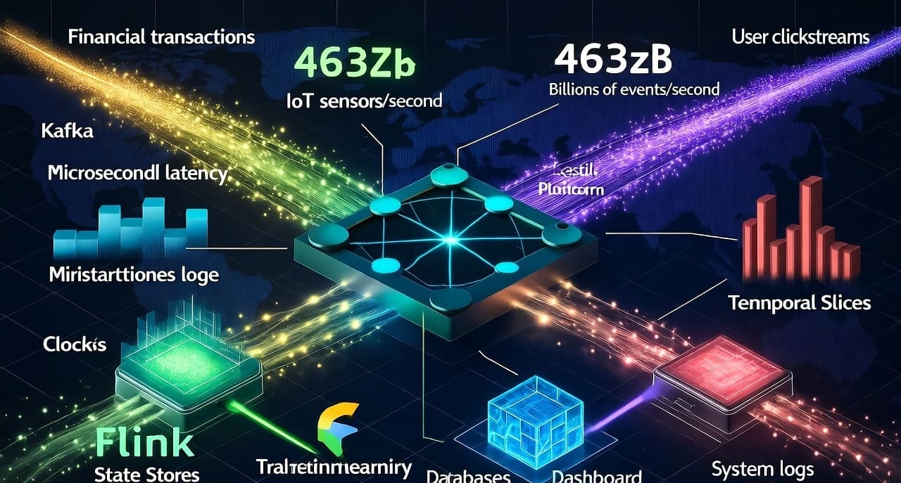
Introduction: The 463 Zettabyte Reality
Every second, millions of IoT sensors transmit temperature readings, thousands of financial transactions execute across global markets, hundreds of thousands of users click through e-commerce sites, and countless mobile apps send telemetry data. By 2025, the world generates an estimated 463 zettabytes of data—a number so staggering it’s nearly incomprehensible. To put it in perspective, that’s equivalent to 463 trillion gigabytes, or enough data to fill 92 billion smartphones every single day.
Here’s the critical insight that’s transforming data engineering: most of this data is born streaming. It doesn’t originate in databases or files—it flows continuously as events, sensor readings, user interactions, and system logs. Yet for decades, we’ve forced this naturally streaming data through batch processing architectures, creating artificial delays, complexity, and missed opportunities.
The question facing data engineers in 2025 isn’t whether to adopt streaming architectures—it’s how to design systems that handle streams natively, efficiently, and reliably at scale. Organizations that master stream processing gain transformative capabilities: detecting fraud in milliseconds rather than hours, personalizing user experiences in real-time rather than overnight, predicting equipment failures minutes before they occur rather than after the fact.
This comprehensive guide explores the complete streaming data ecosystem—from fundamental architectural patterns to practical implementation strategies. Whether you’re a data engineer evaluating Kafka versus Pulsar, an IoT developer building sensor data pipelines, or a platform architect designing real-time analytics infrastructure, you’ll gain actionable insights grounded in production realities rather than theoretical abstractions.
What you’ll learn:
- Core streaming architecture patterns and when to apply them
- The nuanced trade-offs between stream and batch processing
- How to design event-driven systems that scale to billions of events daily
- Practical solutions to streaming’s hardest problems: ordering, exactly-once processing, late data
- Comparative analysis of modern streaming platforms with real-world performance characteristics
- Production patterns for monitoring, debugging, and operating streaming systems
- The emerging convergence of streaming and batch in unified architectures
Understanding Stream Data Models: Events, Messages, and Time
The Fundamental Nature of Streaming Data
Traditional data models assume data exists in persistent storage—rows in databases, files on disks. Stream data models invert this assumption: data is transient by default, flowing continuously through systems. Understanding this fundamental shift is critical to designing effective streaming architectures.
Events as First-Class Citizens:
In streaming systems, the atomic unit is an event—an immutable fact representing something that happened at a specific point in time. Events are fundamentally different from database records:
- Immutability: Events represent facts that occurred; they cannot be “updated” (though new events can supersede prior ones semantically)
- Temporal ordering: Events have inherent time dimensions—when they occurred, when they were observed, when they were processed
- Context independence: Each event should be self-describing, containing all necessary context without requiring lookups to external systems
Consider a simple e-commerce scenario. In a traditional database model, you might update a user’s cart record:
UPDATE shopping_carts
SET items = items + 1, last_updated = NOW()
WHERE user_id = 12345
In a streaming model, you emit events:
{
  "event_type": "item_added_to_cart",
  "event_id": "evt_abc123",
  "user_id": 12345,
  "product_id": 67890,
  "quantity": 1,
  "timestamp": "2025-10-11T14:23:45.123Z",
  "session_id": "sess_xyz789"
}
This seemingly simple shift has profound implications. The event model preserves complete history (every cart addition is recorded, not just current state), enables time-travel queries (what was in the cart at 2 PM?), supports multiple consumers (analytics, recommendations, inventory all process the same event), and allows retroactive processing (new consumers can replay historical events).
The Three Dimensions of Time in Streaming
Time is deceptively complex in streaming systems. Unlike batch processing where time is largely irrelevant (process all data from yesterday), streaming requires careful handling of multiple time dimensions:
Event Time: When the event actually occurred in the real world. A sensor reading at 10:00:00 AM has event time of 10:00:00 AM, regardless of when it’s processed.
Processing Time: When the streaming system processes the event. That same sensor reading might be processed at 10:00:05 AM due to network latency.
Ingestion Time: When the event first entered the streaming system. The sensor reading might reach Kafka at 10:00:02 AM.
The gap between these times creates fundamental challenges:
Latency and Disorder: Network delays, system failures, and distributed processing mean events frequently arrive out of order. An event with event_time of 10:00:00 might arrive after an event with event_time of 10:00:10.
Late Arriving Data: Events can arrive significantly late—sometimes hours or days after their event time. A mobile device might buffer events offline and upload them when connectivity resumes.
Watermarks and Completeness: How do you know when you’ve received “all” events for a given time window? Streaming systems use watermarks—estimates of event-time progress—to trigger computations while acknowledging that late data might still arrive.
Consider aggregating sensor readings per minute. Using processing time is simple but incorrect—slow network means some sensors are underrepresented. Using event time is correct but complex—you must handle out-of-order data, decide when to emit results (after 1 second? 10 seconds? never complete?), and potentially revise results when late data arrives.
Modern streaming frameworks like Apache Flink and Kafka Streams provide sophisticated windowing and watermark mechanisms, but understanding these temporal semantics is essential for correct streaming system design.
Message Semantics and Delivery Guarantees
Streaming systems must handle failures gracefully—network partitions, broker crashes, consumer failures. The guarantee level profoundly impacts both system design and performance:
At-Most-Once Delivery: Events might be lost but are never duplicated. Simple and fast (no persistence required) but unacceptable for most business use cases. Suitable only for non-critical telemetry where occasional data loss is tolerable.
At-Least-Once Delivery: Events are never lost but might be duplicated during failures and retries. The most common guarantee in production—balances reliability with performance. Requires idempotent processing logic (applying the same event twice produces the same result) or deduplication mechanisms.
Exactly-Once Delivery: Events are neither lost nor duplicated—processed exactly once despite failures. The holy grail but expensive to achieve. Requires distributed transactions and coordination, significantly impacting throughput.
The subtle truth: exactly-once processing is often sufficient, but exactly-once delivery is rarely necessary. If your processing logic is idempotent (e.g., writing the same value to a key-value store multiple times), at-least-once delivery with idempotent processing achieves exactly-once semantics at much lower cost.
Core Streaming Architecture Patterns
Pattern 1: Event Streaming Platform (The Central Nervous System)
The most fundamental pattern treats streaming infrastructure as the central integration layer—a distributed log that acts as the system of record for all events.
Architecture Components:
Distributed Log: Kafka, Pulsar, or Kinesis maintains an ordered, replicated, partitioned log of all events. This log is both transport (moving events between systems) and storage (events are retained for hours, days, or indefinitely).
Producers: Applications, services, databases (via change data capture), and external systems publish events to the log.
Consumers: Applications, analytics systems, data warehouses, ML models, and microservices subscribe to event streams and process them independently.
Strengths:
- Decoupling: Producers and consumers are completely independent—adding new consumers doesn’t impact existing systems
- Scalability: Partitioning enables horizontal scaling to billions of events per day
- Replayability: Consumers can reprocess historical events, enabling schema evolution, bug fixes, and new analytics retroactively
- Durability: Events are persisted and replicated, surviving individual component failures
Challenges:
- Ordering complexity: Maintaining order across partitions requires careful partition key design
- Schema evolution: Changes to event schemas must be managed carefully to avoid breaking consumers
- Operational overhead: Operating Kafka or Pulsar clusters requires specialized expertise
- Cost at scale: Retaining large event histories (especially with high replication factors) can be expensive
When to Use:
This pattern excels for organizations with multiple systems that need to share data in real-time, event-driven microservices architectures, and scenarios requiring both real-time processing and historical replay. It’s the foundation for most modern streaming architectures.
Production Example:
A retail organization uses Kafka as their central event streaming platform. Point-of-sale systems publish transaction events, inventory systems publish stock-level changes, and customer service systems publish interaction events. These streams feed:
- Real-time dashboards showing current sales by region
- Fraud detection ML models analyzing transaction patterns
- Inventory optimization systems triggering restock orders
- Customer data platforms building unified customer profiles
- Data lake for historical analysis and reporting
Each consumer processes events independently, and new use cases are enabled by simply adding new consumers to existing streams—no changes to source systems required.
Pattern 2: Stream Processing Applications (Continuous Transformations)
This pattern focuses on applications that continuously transform streaming data—filtering, aggregating, joining, and enriching events as they flow through the system.
Architecture Components:
Stream Processing Framework: Flink, Kafka Streams, Spark Streaming, or cloud-native services (Kinesis Data Analytics, Dataflow) provide the runtime for transformation logic.
State Management: Stateful processing (aggregations, joins, deduplication) requires distributed state stores that survive failures and scale horizontally.
Windowing Logic: Time-based or count-based windows define boundaries for aggregations and joins in infinite streams.
Strengths:
- Low latency: Process events within milliseconds of arrival
- Complex transformations: Support sophisticated logic including stateful aggregations, stream-stream joins, and temporal patterns
- Scalability: Modern frameworks handle millions of events per second across distributed clusters
- Fault tolerance: State is checkpointed and can be recovered after failures
Challenges:
- State management complexity: Large state sizes can impact performance and recovery time
- Late data handling: Deciding how long to wait for late-arriving events requires careful tuning
- Debugging difficulty: Distributed streaming applications are inherently harder to debug than batch jobs
- Resource management: Streaming applications run continuously, requiring always-on infrastructure
When to Use:
Apply this pattern for real-time aggregations (metrics, dashboards), event enrichment (joining streams with reference data), complex event processing (pattern detection, anomaly identification), and continuous ETL (transforming events before loading to warehouses or lakes).
Production Example:
A financial services firm uses Flink to process market data feeds. The application:
- Ingests millions of trade and quote events per second from exchanges
- Enriches trades with reference data (security details, exchange information)
- Computes rolling aggregations (minute-level VWAP, trading volumes by security)
- Detects patterns indicating market manipulation or suspicious trading
- Publishes enriched events to downstream risk management systems
The entire pipeline operates with sub-100ms latency, enabling traders and risk managers to make decisions on current market conditions rather than delayed snapshots.
Pattern 3: Change Data Capture (CDC) Streaming
CDC patterns treat databases as event sources, capturing every insert, update, and delete as events in a stream. This bridges traditional database systems with modern streaming architectures.
Architecture Components:
CDC Tools: Debezium, Maxwell, Oracle GoldenGate, or native database features (PostgreSQL logical replication, MySQL binlog) capture database changes.
Event Transformation: CDC events are often translated from database-specific formats into domain events meaningful to business applications.
Downstream Consumers: Multiple systems consume the change stream for different purposes—search indexes, cache invalidation, analytics, data replication.
Strengths:
- No application changes: Capture data changes without modifying existing applications
- Complete data history: Every change is captured, enabling temporal queries and audit trails
- Consistency: Changes are captured in transaction order, preserving referential integrity
- Multiple consumers: Single change stream serves many downstream needs
Challenges:
- Schema dependencies: Consumers depend on database schemas, which may not represent ideal domain models
- Delete handling: Capturing deletions requires careful design—soft deletes or tombstone events
- Large transactions: Very large database transactions can create oversized CDC events
- Operational coupling: Database performance and availability impacts CDC pipeline
When to Use:
CDC shines for incrementally loading data warehouses and lakes, maintaining search indexes (Elasticsearch, Solr) in sync with databases, invalidating caches when data changes, and replicating data across regions or systems without dual-writes in application code.
Production Example:
An e-commerce platform uses Debezium to capture changes from their PostgreSQL order database. The CDC stream:
- Updates the Elasticsearch product catalog within seconds of inventory changes
- Invalidates Redis cache entries when orders are placed or cancelled
- Feeds real-time analytics dashboards showing order volumes and revenue
- Loads incrementally to Snowflake for business intelligence
- Triggers order fulfillment workflows in downstream microservices
This architecture eliminates complex polling queries, reduces database load, and ensures all systems see consistent, timely data without custom integration code in the order service.
Pattern 4: Lambda Architecture (Hybrid Batch and Streaming)
Lambda architecture attempts to balance streaming’s low latency with batch processing’s accuracy and ease of implementation by maintaining parallel batch and streaming pipelines.
Architecture Components:
Batch Layer: Processes complete historical datasets periodically (hourly, daily) using batch frameworks (Spark, Presto), producing accurate “batch views.”
Speed Layer: Processes recent data in real-time using streaming frameworks, producing approximate “real-time views.”
Serving Layer: Merges batch and real-time views, presenting unified results to applications and users.
Strengths:
- Accuracy and latency trade-off: Get fast approximate answers while batch processing computes accurate results
- Reprocessing capability: Batch layer can reprocess historical data when logic changes
- Fault tolerance: Streaming failures don’t prevent accurate batch results from eventually appearing
Challenges:
- Operational complexity: Maintaining two separate pipelines with different frameworks doubles development and operational burden
- Code duplication: Business logic must be implemented twice (batch and streaming), creating consistency risks
- Query complexity: Applications must understand how to merge batch and real-time views
- Cost inefficiency: Running parallel pipelines consumes more resources than unified approaches
When to Use:
Lambda is most appropriate when accuracy is critical but latency requirements exist (financial reporting with real-time previews), when streaming technology is immature or unproven in your organization, or during transitions from batch to streaming (run parallel systems while building confidence).
Production Example:
A social media analytics platform uses Lambda architecture for engagement metrics. The streaming layer (Kafka Streams) computes approximate engagement counts (likes, shares, comments) within seconds for dashboards. The batch layer (Spark) reprocesses the same data overnight, correcting for duplicates, spam, and late-arriving data. Users see real-time estimates that are replaced by accurate counts the next morning.
However, this organization is now actively migrating to Kappa architecture (explained next) because maintaining duplicate logic across streaming and batch pipelines created persistent bugs and doubled engineering effort.
Pattern 5: Kappa Architecture (Streaming-First)
Kappa architecture simplifies Lambda by eliminating the batch layer—using a single streaming pipeline for both real-time and historical processing. Reprocessing is achieved by replaying the event stream from earlier points.
Architecture Components:
Unified Processing Framework: A single streaming framework (typically Flink or Kafka Streams) handles both real-time and reprocessing workloads.
Immutable Event Log: Events are retained indefinitely (or for very long periods), enabling complete reprocessing when needed.
Versioned Consumers: Multiple versions of processing applications can run simultaneously during migrations or A/B testing.
Strengths:
- Simplified architecture: Single codebase, single framework, single operational model
- Consistency: Real-time and historical views use identical logic, eliminating discrepancies
- Efficiency: No duplicate processing of historical data unless explicitly reprocessing
- Agility: Faster iteration when changes require only one pipeline modification
Challenges:
- Stream retention costs: Storing events indefinitely can be expensive for high-volume streams
- Reprocessing time: Replaying months of events can take hours or days
- State management: Very large state (e.g., billions of user profiles) can be challenging to bootstrap
- Framework dependency: Organizational success depends heavily on the chosen streaming framework’s maturity
When to Use:
Kappa is ideal for organizations with streaming-first culture, scenarios where most data is born streaming (IoT, clickstreams, application events), and when agility is valued over the safety net of parallel batch processing. It represents the modern best practice for greenfield architectures.
Production Example:
A logistics company uses Kappa architecture for shipment tracking. All tracking events (package scanned, departed facility, out for delivery) flow through Kafka. A single Flink application processes these events to:
- Update current shipment status for customer-facing tracking dashboards
- Compute aggregate metrics (on-time delivery rates, facility throughput)
- Detect anomalies (unusual delays, missing scans)
When they need to change the logic (e.g., update how “delivered late” is defined), they deploy a new version of the Flink application and replay the last month of events from Kafka to recompute historical metrics with the new definition. This takes 4 hours but requires zero additional code compared to Lambda architecture’s separate batch implementation.
Stream vs Batch: Making the Right Trade-Off
The streaming versus batch decision is nuanced—not a binary choice but a spectrum of trade-offs. Understanding when each approach (or hybrid approaches) is appropriate requires analyzing multiple dimensions.
Latency Requirements: The Primary Decision Driver
When Streaming is Essential (Sub-Second to Seconds Latency):
- Fraud detection in financial transactions (must block fraudulent transactions before completion)
- Real-time personalization (recommend products based on current browse session)
- Infrastructure monitoring and alerting (detect and respond to outages within seconds)
- Algorithmic trading and market data analysis
- IoT anomaly detection (identify equipment failures before catastrophic damage)
When Batch is Sufficient (Minutes to Hours Latency):
- Regulatory reporting (daily/monthly submissions)
- Executive dashboards (updated overnight)
- Historical trend analysis and forecasting
- Data warehouse loading for business intelligence
- Batch ML model training on large datasets
The 15-Minute Rule: Many organizations find that if results can wait 15 minutes, micro-batch processing (Spark Streaming in batch mode, scheduled workflows every 15 minutes) offers a pragmatic middle ground—near-real-time results with batch simplicity.
Complexity and Development Velocity
Batch Advantages:
- Simpler mental model: Process complete datasets with well-defined boundaries
- Easier debugging: Can examine intermediate outputs, rerun failed jobs, inspect data at any stage
- Mature ecosystems: Extensive libraries, tools, and community knowledge
- Forgiving error handling: Jobs can be retried, manual fixes applied to output
Streaming Complexity:
- Distributed state management: Maintaining state across partitions and surviving failures is inherently complex
- Time and windowing: Handling out-of-order events and late data requires careful design
- Continuous operation: No clear start/end, making testing and validation challenging
- Cascading failures: Errors can compound across pipeline stages without careful monitoring
Organizations with limited streaming expertise should start with batch and selectively adopt streaming for high-value use cases. Attempting to build streaming-first architectures without foundational skills leads to reliability issues and costly failures.
Cost Considerations
Streaming Costs:
- Always-on infrastructure: Streaming applications run 24/7, even during low-traffic periods
- State storage: Large stateful applications require fast storage (SSDs, memory), driving costs
- Over-provisioning: Must handle peak load, leading to underutilization during normal periods
- Operational complexity: Requires specialized expertise, increasing labor costs
Batch Costs:
- Efficient resource usage: Jobs run only when needed, shutting down afterward
- Cheaper storage: Can use S3/ADLS for intermediate data rather than expensive hot storage
- Simpler operations: Easier to troubleshoot and maintain with smaller ops teams
Cost-Effectiveness Crossover: Streaming becomes cost-competitive when data velocity is high and consistent. If you’re processing data continuously throughout the day anyway, streaming’s always-on infrastructure isn’t wasteful. But for bursty workloads (process once daily at 2 AM), batch is far more economical.
A financial services firm found that streaming became more cost-effective than batch when processing frequency exceeded every 30 minutes. Below that threshold, the overhead of keeping streaming infrastructure running outweighed batch job startup costs.
Data Characteristics
Favor Streaming When:
- Data is naturally streaming: IoT sensors, user clickstreams, application logs
- Event order matters: Processing sequence affects results
- Temporal relationships important: Detecting patterns across time windows
- Data has short shelf-life: Real-time offers, time-sensitive alerts
Favor Batch When:
- Data arrives in bulk: Daily file drops, database exports, third-party data deliveries
- Processing requires complete datasets: Machine learning training, complex analytics requiring full history
- Results are aggregations: Daily summaries, monthly reports
- Reprocessing is common: Frequent logic changes require recomputing historical results
The Hybrid Reality
Most organizations run hybrid architectures—streaming for operational use cases (monitoring, real-time features) and batch for analytical workloads (reporting, ML training). The key is avoiding unnecessary streaming complexity where batch suffices while ensuring latency-sensitive workloads leverage streaming’s strengths.
Hybrid Pattern Example:
A ride-sharing platform uses:
- Streaming for driver-rider matching, real-time ETAs, surge pricing (seconds latency)
- Micro-batch (5-minute windows) for operational dashboards, city-level demand heatmaps
- Batch (nightly) for driver earnings calculations, rider billing, data warehouse loading
This pragmatic approach delivers real-time capabilities where they create user value while controlling costs and complexity for less time-sensitive workloads.
Scalability: Handling Billions of Events Daily
Partitioning Strategies for Horizontal Scale
Streaming systems achieve massive scalability through partitioning—splitting event streams across multiple parallel processing units. Effective partitioning is critical for both performance and correctness.
Partition Key Selection:
The partition key determines which events go to which partition. This seemingly simple choice has cascading implications:
Random Partitioning: Maximizes load balance but destroys event ordering. Suitable only when order is completely irrelevant (rare in practice).
Key-Based Partitioning: Events with the same key always go to the same partition, preserving per-key ordering. The standard approach for most use cases.
Time-Based Partitioning: Events are partitioned by timestamp, useful for time-series data but can create hot partitions (all current events go to one partition).
Custom Partitioning: Application-specific logic—for example, geographic partitioning (all California events to partition A) or tenant-based partitioning in multi-tenant systems.
Common Partition Key Pitfalls:
- Hot Keys: If a small number of keys account for most events (think celebrity user_ids), those partitions become bottlenecks. Solution: composite keys or sub-partitioning highly active keys.
- Cardinality Mismatch: Too few unique keys for number of partitions wastes parallelism. Too many keys for consumer capacity overwhelms downstream systems.
- Key Skew Over Time: Partition keys that were balanced initially become skewed as usage patterns change (e.g., new users concentrated in specific cohorts).
Real-World Partitioning Example:
A gaming platform initially partitioned player events by user_id, which worked well until certain players (streamers with millions of viewers) generated 1000x more events than typical players. They redesigned partitioning to use hash(user_id + session_id), spreading each player’s events across multiple partitions while maintaining session-level ordering. This prevented hot partitions while preserving the ordering guarantees their analytics required.
Backpressure and Flow Control
When downstream consumers can’t keep up with data production rates, backpressure mechanisms prevent catastrophic system failures. Understanding and implementing backpressure is critical for production streaming systems.
Backpressure Strategies:
Buffering: Store excess events in memory or disk buffers temporarily. Simple but has limits—if consumers never catch up, buffers eventually fill and overflow.
Dropping: Discard events when capacity is exceeded. Acceptable for telemetry and non-critical events but catastrophic for financial transactions. Requires explicit business approval.
Blocking Producers: Stop or slow event production until consumers catch up. Maintains data integrity but can cascade backwards, impacting source systems.
Dynamic Scaling: Auto-scale consumer capacity when queues grow. The ideal solution but requires infrastructure sophistication and can’t scale infinitely.
Load Shedding: Intelligently drop low-priority events while preserving critical ones. Requires event prioritization metadata and sophisticated coordination.
Production Backpressure Example:
An e-commerce platform experiences traffic spikes during flash sales—10x normal event rates within seconds. Their streaming architecture handles this through:
- Kafka buffering: Brokers buffer events for minutes while consumers scale up
- Kubernetes auto-scaling: Consumer pods scale from 10 to 100 based on consumer lag metrics
- Graceful degradation: Non-critical analytics consumers pause during spikes, allowing critical real-time features (cart, checkout) to maintain performance
- Proactive alerts: Operations receive warnings when consumer lag exceeds 1 minute, enabling manual intervention if auto-scaling is insufficient
This multi-layered approach prevents outages while ensuring business-critical functions remain operational under extreme load.
State Management at Scale
Stateful stream processing—maintaining aggregations, session windows, join state—becomes challenging at scale. State sizes can reach terabytes, requiring sophisticated management strategies.
State Storage Options:
In-Memory State: Fastest but limited by RAM capacity and expensive. Suitable for small state (< 100 GB per node) with frequent access.
Local Disk State: RocksDB (used by Flink and Kafka Streams) provides durable, disk-backed state with acceptable performance. Can handle hundreds of GB per node.
Remote State: Store state in external systems (Redis, DynamoDB). Slower but enables independent state scaling. Suitable for infrequently accessed or enormous state.
Tiered State: Hot state in memory, warm state on local disk, cold state remotely. Provides balance of performance and scalability.
State Partitioning: State is partitioned alongside data—each processing unit manages state only for its assigned partition keys. This enables horizontal scaling but complicates operations like repartitioning.
Checkpointing for Fault Tolerance:
Streaming frameworks periodically checkpoint state to durable storage (S3, HDFS). If a processing node fails, state is recovered from the last checkpoint. The checkpoint frequency represents a trade-off:
- Frequent checkpoints (every 30 seconds): Minimal data reprocessing after failures but high I/O overhead
- Infrequent checkpoints (every 10 minutes): Lower overhead but more reprocessing and longer recovery times
State Management Example:
A fraud detection system maintains user behavioral profiles (average transaction amount, typical merchant categories, geographic patterns) as state. With 500 million users and 2KB per profile, total state is 1TB.
They manage this by:
- Partitioning state across 50 Flink task managers (20GB each)
- Using RocksDB for local state storage on fast SSDs
- Checkpointing to S3 every 5 minutes (full checkpoint takes 90 seconds)
- Implementing incremental checkpoints (only changed state) to reduce I/O
- Monitoring state size growth and alerting when individual partitions exceed 30GB
This architecture handles 50,000 transactions/second while maintaining sub-200ms latency for fraud scoring.
Platform Comparison: Kafka, Pulsar, Kinesis, and Beyond
Apache Kafka: The Industry Standard
Kafka dominates the streaming platform landscape, powering event infrastructure at the majority of large enterprises. Understanding its strengths and limitations informs architectural decisions.
Strengths:
Massive Ecosystem: Kafka Connect (hundreds of source/sink connectors), Kafka Streams, ksqlDB, Schema Registry, and extensive third-party integrations make Kafka a complete streaming platform beyond just message transport.
Proven Scalability: LinkedIn processes trillions of messages daily through Kafka. The architecture scales horizontally to handle virtually any throughput requirement.
Operational Maturity: Decade-long production use means edge cases are well-understood, failure modes documented, and operations playbooks extensive.
Multi-Tenancy: Single Kafka cluster can serve dozens of applications with isolation through ACLs, quotas, and separate topics.
Limitations:
Operational Complexity: Running production Kafka clusters requires deep expertise. Zookeeper management (being phased out with KRaft mode), broker rebalancing, and partition management have learning curves.
Rebalancing Disruptions: Consumer group rebalancing (when consumers join/leave) causes brief processing pauses. For latency-sensitive applications, this can be problematic.
Storage Inefficiency: Kafka stores complete messages even when consumers only need subsets. For large events (documents, images), this can be wasteful.
Limited Multi-Datacenter: While Kafka replication works well within clusters, cross-datacenter replication (MirrorMaker 2) is a separate concern with additional complexity.
When to Choose Kafka:
Kafka is the safe, default choice for most streaming needs. Its maturity, ecosystem, and talent availability make it appropriate for the majority of use cases. Choose Kafka unless you have specific requirements it doesn’t meet well (massive geo-distribution, complex message routing, tight cloud integration).
Apache Pulsar: The Multi-Tenant Alternative
Pulsar emerged from Yahoo’s need for truly multi-tenant, globally distributed messaging. It architectural differences from Kafka make it superior for specific use cases.
Architectural Differences:
Separation of Storage and Serving: Kafka brokers handle both message serving and storage. Pulsar separates these—bookies store data while brokers serve it. This enables independent scaling of storage and serving capacity.
Native Multi-Tenancy: Pulsar was designed from the ground up for multi-tenancy with namespaces, separate
authentication per tenant, and resource quotas. Kafka added these later and they’re less polished.
Geo-Replication: Pulsar’s built-in geo-replication is more sophisticated than Kafka’s, handling cross-cluster replication transparently with conflict resolution.
Strengths:
Cloud-Native Architecture: Pulsar’s design fits cloud environments naturally—storage on object stores (S3), compute on Kubernetes, seamless scaling.
Infinite Retention: Because storage is separate and uses cheap object storage, Pulsar can retain messages indefinitely without expensive broker disk.
Flexible Messaging: Supports both streaming (Kafka-like) and queuing semantics (RabbitMQ-like) in one platform.
Limitations:
Smaller Ecosystem: Fewer connectors, less tooling, smaller community than Kafka. You’ll often need to build custom solutions.
Operational Immaturity: Fewer production war stories, edge cases less documented, operations expertise harder to find.
Performance Gaps: While Pulsar scales well, Kafka’s single-node throughput is typically higher for simple use cases.
When to Choose Pulsar:
Pulsar shines for multi-tenant SaaS platforms (each customer gets isolated namespace), global deployments requiring sophisticated geo-replication, cloud-native environments leveraging Kubernetes and object storage, or when infinite retention is critical (compliance, audit, reprocessing).
AWS Kinesis: The Managed Cloud Option
Kinesis offers fully managed streaming for AWS-centric organizations willing to accept some architectural trade-offs for operational simplicity.
Strengths:
Zero Operations: AWS manages all infrastructure—no brokers to patch, no capacity planning, no Zookeeper debugging.
AWS Integration: Native integration with Lambda, Firehose, Analytics, S3—building AWS-native streaming pipelines is straightforward.
Instant Scaling: Add shards instantly without rebalancing delays or cluster reconfiguration.
Security: Integrates seamlessly with IAM, KMS, VPC—security is simple compared to self-managed Kafka.
Limitations:
Cost at Scale: Kinesis pricing (per shard-hour plus data ingestion) becomes expensive at high volumes. Organizations processing TBs daily often find Kafka more economical.
Shard Limits: Maximum 1MB/sec write and 2MB/sec read per shard. High-velocity streams require many shards, increasing costs and operational complexity.
Retention Limits: Default 24 hours, max 365 days. Much shorter than Kafka’s indefinite retention.
AWS Lock-In: Migrating away from Kinesis to multi-cloud or on-premises is difficult.
When to Choose Kinesis:
Kinesis is ideal for AWS-only organizations, moderate data volumes (< 10 TB/day), teams without dedicated streaming platform expertise, or prototypes and MVPs where time-to-market matters more than long-term cost optimization.
Platform Selection Matrix
| Requirement | Kafka | Pulsar | Kinesis | Kafka on Cloud (MSK, Confluent Cloud) |
|---|---|---|---|---|
| Multi-cloud strategy | Excellent | Excellent | Poor (AWS only) | Good |
| Operational simplicity | Poor (self-managed) | Poor (self-managed) | Excellent | Good |
| Cost at scale (>10TB/day) | Excellent | Good | Poor | Good |
| Ecosystem maturity | Excellent | Moderate | Good (AWS) | Excellent |
| Multi-tenancy | Good | Excellent | Moderate | Good |
| Geo-replication | Moderate | Excellent | Moderate | Good |
| Talent availability | Excellent | Poor | Good | Excellent |
Excellent | | Time to production | Moderate | Moderate | Fast | Fast | | Infinite retention | Good | Excellent | Poor | Good | | Performance (single-node) | Excellent | Good | Moderate | Excellent |
Stream Processing Frameworks: Flink, Spark, and Kafka Streams
Apache Flink: The True Streaming Engine
Flink represents the state-of-the-art in stream processing—designed from the ground up for continuous, stateful computations over unbounded data streams.
Core Architectural Advantages:
True Streaming Model: Unlike Spark Streaming’s micro-batches, Flink processes events individually as they arrive. This enables true millisecond latency and makes the programming model more intuitive.
Advanced State Management: Flink’s state handling is sophisticated—distributed snapshots (Chandy-Lamport algorithm) enable exactly-once processing guarantees while maintaining high throughput.
Event Time Processing: First-class support for event time, watermarks, and late data handling. Flink’s windowing semantics are more powerful and correct than alternatives.
SQL Support: Flink SQL enables declarative stream processing for analysts and less engineering-intensive use cases. The SQL layer can express complex streaming operations including temporal joins and pattern matching.
Strengths:
Low Latency: Sub-second latency for most operations, millisecond latency for simple transformations. Superior to Spark Streaming for latency-sensitive workloads.
Exactly-Once Guarantees: End-to-end exactly-once processing across sources, transformations, and sinks (when supported). Critical for financial and transactional use cases.
Complex Event Processing: Pattern detection, sessionization, and temporal joins are first-class operations in Flink’s API.
Batch Unification: Flink treats batch as a special case of streaming (bounded streams), enabling unified codebase for both workloads.
Limitations:
Operational Complexity: Running production Flink requires expertise in distributed systems, checkpoint tuning, state backend configuration, and resource management.
Smaller Ecosystem: Fewer pre-built connectors compared to Spark. You’ll often write custom sources and sinks.
Resource Requirements: Flink’s always-on model and stateful processing require substantial infrastructure even for modest workloads.
Debugging Challenges: Distributed streaming applications with event-time semantics are inherently difficult to debug and test.
When to Choose Flink:
Flink is the right choice for latency-critical applications (fraud detection, real-time recommendations), complex event processing (pattern detection, temporal analytics), exactly-once requirements (financial transactions), or when event-time correctness is paramount (out-of-order data, late arrivals). Organizations building streaming-first architectures should seriously consider Flink despite its learning curve.
Production Example:
A telecommunications company uses Flink for network monitoring across 50 million connected devices. Their Flink application:
- Ingests 2 million events per second from network equipment
- Maintains per-device state (connection quality metrics, recent error patterns)
- Detects anomalies using complex temporal patterns (specific error sequences indicating hardware failure)
- Triggers automated remediation workflows within 500ms of detecting critical issues
- Scales across 200 Flink task managers processing 8TB of data daily
This level of real-time sophistication with exactly-once guarantees would be extremely difficult with alternative frameworks.
Apache Spark Streaming: The Batch-Streaming Hybrid
Spark Streaming (and its evolution, Structured Streaming) brings Spark’s powerful batch processing capabilities to streaming workloads through micro-batch processing.
Architectural Model:
Spark Streaming divides continuous streams into small batches (typically 1-10 seconds), processing each batch using Spark’s familiar RDD/DataFrame APIs. This micro-batch approach bridges batch and streaming paradigms.
Strengths:
Unified API: Identical DataFrame/Dataset API for batch and streaming. Teams skilled in Spark batch can adopt streaming with minimal learning curve.
Ecosystem Integration: Leverage Spark’s massive ecosystem—ML libraries, graph processing, SQL analytics—all work with streaming data.
Throughput Optimization: Micro-batching enables batch-oriented optimizations (query plan optimization, whole-stage code generation) that can achieve higher throughput than event-at-a-time processing.
Simplified Operations: If you’re already running Spark clusters for batch jobs, adding streaming workloads uses the same infrastructure and operational expertise.
Fault Tolerance: Spark’s lineage-based fault tolerance (recompute lost partitions from source) is simpler to understand than Flink’s checkpoint/savepoint model.
Limitations:
Latency Floor: Micro-batch model imposes minimum latency equal to batch interval. Sub-second latency is difficult to achieve without extreme tuning.
State Management: While Structured Streaming added stateful operations, state handling is less sophisticated than Flink—larger state sizes can cause performance issues.
Incremental Processing: Micro-batches are processed atomically, making truly incremental computations (updating state as each event arrives) awkward.
Resource Efficiency: Spark’s overhead makes it less efficient than Flink for simple transformations on modest data volumes.
When to Choose Spark Streaming:
Spark Streaming fits organizations with existing Spark expertise and infrastructure, workloads where 1-10 second latency is acceptable, use cases requiring Spark’s ML/graph capabilities on streaming data, or when unified batch and streaming code is valued over absolute performance.
Production Example:
A media streaming service uses Spark Structured Streaming for user engagement analytics. Their pipeline:
- Processes clickstream events in 5-second micro-batches (500K events per batch)
- Computes session-level metrics (watch time, content viewed, engagement scores)
- Joins streaming events with batch-loaded content metadata (titles, genres, cast)
- Updates session state maintained in Delta Lake
- Feeds real-time dashboards showing current viewership by content and region
The 5-second latency is acceptable for their dashboards, and using Spark enables their data scientists to use the same MLlib models for batch training and streaming scoring without code changes.
Kafka Streams: The Lightweight Library
Kafka Streams is fundamentally different from Flink and Spark—it’s a Java library embedded in applications rather than a separate cluster framework. This architectural choice has profound implications.
Architectural Model:
Kafka Streams applications are standard Java/Scala applications that happen to process Kafka streams. No separate cluster, no external resource manager—just regular microservices that connect to Kafka.
Strengths:
Operational Simplicity: Deploy as standard applications—Docker containers, Kubernetes pods, or traditional servers. No separate streaming cluster to manage.
Lightweight: Minimal resource overhead. Applications can be small, single-purpose microservices rather than monolithic streaming jobs.
Kafka Integration: Trivial to use Kafka-specific features (headers, transactions, consumer groups). The integration is seamless because it’s the same ecosystem.
Exactly-Once Semantics: Kafka Streams provides exactly-once processing using Kafka transactions—simpler to configure than Flink’s checkpointing.
Elastic Scalability: Scale by adding application instances. Kafka’s consumer group protocol handles load distribution automatically.
Limitations:
Kafka Dependency: Completely tied to Kafka—can’t process from Pulsar, Kinesis, or custom sources without workarounds.
JVM Only: Native support only for Java/Scala. Other languages require separate implementations or wrappers.
Limited Windowing: Windowing capabilities are less sophisticated than Flink—complex temporal operations are harder to express.
State Limitations: State stores are local RocksDB instances. Very large state (>100GB per instance) can cause performance and operational issues.
When to Choose Kafka Streams:
Kafka Streams excels for Kafka-centric architectures, microservices-style streaming applications (each service processes its own streams), organizations without streaming cluster expertise, or when operational simplicity is paramount. It’s the right choice for simpler transformations and aggregations where Flink’s power isn’t needed.
Production Example:
An e-commerce platform uses Kafka Streams for product recommendation scoring. They deploy 20 independent Kafka Streams microservices, each consuming user interaction events and computing different recommendation signals:
- Recent view history similarity
- Purchase pattern matching
- Category affinity scoring
- Time-based trending factors
Each microservice runs as a Kubernetes deployment with 3-5 pods, auto-scaling based on Kafka consumer lag. The architecture is simple to operate—standard microservice deployment and monitoring—without requiring streaming cluster expertise. When they need to add new recommendation signals, they deploy another microservice without impacting existing ones.
Framework Selection Decision Tree
Choose Flink if:
- You need sub-second latency consistently
- Exactly-once processing is critical (financial, transactional)
- Complex event processing, pattern detection, or sophisticated windowing is required
- Event-time correctness matters (out-of-order data, late arrivals)
- You have streaming infrastructure expertise or willingness to invest in developing it
Choose Spark Streaming if:
- 1-10 second latency is acceptable
- You need unified batch and streaming code
- Existing Spark infrastructure and expertise
- ML/graph processing on streaming data required
- Batch-style optimizations (whole-stage codegen) benefit your workload
Choose Kafka Streams if:
- Microservices architecture with Kafka already central
- Operational simplicity more important than maximum performance
- Modest state requirements (<50GB per instance)
- Standard application deployment preferred over cluster management
- JVM languages acceptable (Java, Scala, Kotlin)
Production Patterns: Monitoring, Debugging, and Operations
The Observability Challenge
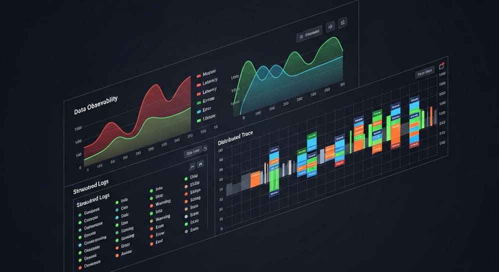
Streaming systems are inherently difficult to observe—data flows continuously, state is distributed, and failures manifest in subtle ways (gradually increasing lag, silent data loss, incorrect aggregations). Comprehensive observability is essential for production reliability.
Critical Metrics to Monitor:
Throughput Metrics:
- Events per second ingested (by source, topic, partition)
- Events per second processed (by transformation, operator)
- End-to-end throughput (source to sink)
- Backpressure indicators (buffer sizes, blocked producers)
Latency Metrics:
- Event time to processing time lag (how far behind is processing?)
- Per-stage processing latency (identify bottlenecks)
- End-to-end latency (source event to sink commit)
- Watermark lag (how far behind is the watermark from current time?)
Error Metrics:
- Processing errors (failed transformations, exceptions)
- Data quality issues (schema validation failures, null values in required fields)
- Consumer lag (events waiting to be processed)
- Checkpoint/commit failures
Resource Metrics:
- CPU utilization per processing unit
- Memory usage (heap, off-heap for RocksDB)
- Disk I/O (for state backends)
- Network bandwidth (between processing stages)
Business Metrics:
- Domain-specific metrics embedded in streams (transaction amounts, error rates, user actions)
- Data freshness (time since last event processed for critical streams)
- Completeness (expected vs. actual event counts)
Observability Stack Example:
A financial services firm’s streaming observability architecture:
Metrics Collection: Prometheus scrapes metrics from Flink job managers and Kafka exporters every 15 seconds Dashboards: Grafana dashboards showing real-time processing rates, lag, error rates, and resource utilization Alerting: Alert manager triggers pages for consumer lag >5 minutes, error rates >0.1%, or watermark lag >10 minutes Distributed Tracing: OpenTelemetry traces follow individual transactions through the streaming pipeline, identifying bottlenecks Log Aggregation: ELK stack collects application logs, enabling error investigation and pattern detection Business Metrics: Custom metrics embedded in streams track critical KPIs (trade execution latency, market data freshness)
This comprehensive observability enabled them to detect and resolve a subtle issue where specific partition keys caused 2x processing latency—identified through distributed tracing showing one partition’s events consistently taking longer to process.
Debugging Streaming Applications
Debugging distributed streaming systems requires different approaches than traditional applications—you can’t simply add breakpoints and step through code.
Effective Debugging Techniques:
Data Sampling: Extract representative samples from streams for local testing. Process these samples through your pipeline in a controlled environment to reproduce issues.
Shadow Streams: Duplicate production streams to test environments. Run experimental pipeline versions against real data without impacting production.
Replay Testing: Capture and replay production events through development pipelines. This allows iterative debugging with deterministic inputs.
State Inspection: Export and examine state stores offline. For RocksDB-backed state, extract snapshots and query them with custom tools to understand why state is growing or containing unexpected values.
Time Travel: Use Kafka’s offset management to reprocess historical data. When bugs are fixed, replay events to regenerate correct outputs.
Synthetic Events: Inject tagged test events into production streams. Track these known events through the pipeline to validate end-to-end behavior.
Debugging War Story:
A rideshare platform experienced puzzling issues where driver availability estimates were occasionally wrong—showing drivers as available when they’d already accepted rides. Debugging revealed:
- Symptoms: Random availability inaccuracies affecting <1% of requests
- Initial hypothesis: Race conditions in state updates (wrong)
- Debugging approach: Injected synthetic driver state change events with unique identifiers
- Discovery: Traced synthetic events revealed occasional out-of-order processing when partition rebalancing occurred
- Root cause: Their processing logic assumed in-order delivery within partitions, but during rebalancing, buffered events could arrive late
- Solution: Added event sequence numbers and reordered buffered events before processing
This issue would have been nearly impossible to debug without the ability to inject synthetic events and trace them through the pipeline.
Handling Schema Evolution
As streaming systems evolve, event schemas inevitably change—new fields added, types modified, semantics updated. Managing schema evolution without breaking downstream consumers is critical.
Schema Evolution Strategies:
Forward Compatibility: New producers can write schemas that old consumers can read (typically by making new fields optional)
Backward Compatibility: Old producers’ schemas can be read by new consumers (new consumers handle missing fields gracefully)
Full Compatibility: Both forward and backward compatible—the gold standard but most restrictive
Schema Registry Pattern: Centralize schema management in a registry (Confluent Schema Registry, AWS Glue Schema Registry). Producers register schemas before use, consumers fetch schemas dynamically.
Practical Evolution Patterns:
Adding Optional Fields: Always safe—old consumers ignore new fields, new consumers use defaults when fields are missing
Removing Fields: Announce deprecation period, monitor usage, remove only after all consumers updated
Changing Types: Generally breaking—prefer adding new fields with new types and deprecating old fields
Renaming Fields: Breaking—treat as remove-and-add operation with transition period
Schema Evolution Example:
An IoT platform evolved their sensor event schema:
Version 1 (Initial):
{
  "sensor_id": "sens_12345",
  "temperature": 72.5,
  "timestamp": "2025-10-11T10:00:00Z"
}
Version 2 (Add humidity, optional):
{
  "sensor_id": "sens_12345",
  "temperature": 72.5,
  "humidity": 45.2,  // NEW: optional field
  "timestamp": "2025-10-11T10:00:00Z"
}
Version 3 (Add location, change temperature precision):
{
  "sensor_id": "sens_12345",
  "temperature_celsius": 72.48,  // NEW: higher precision, new field name
  "temperature": 72.5,  // DEPRECATED: maintained for backward compatibility
  "humidity": 45.2,
  "location": {"lat": 37.7749, "lon": -122.4194},  // NEW: optional
  "timestamp": "2025-10-11T10:00:00Z"
}
They maintained both temperature and temperature_celsius for 6 months while consumers migrated, then deprecated temperature. This gradual evolution prevented breaking any downstream systems.
Disaster Recovery and Failure Handling
Streaming systems must gracefully handle failures at every level—individual event processing errors, processing node failures, broker outages, and complete data center failures.
Multi-Level Failure Strategies:
Event-Level Errors (malformed data, processing exceptions):
- Dead letter queues (DLQs) capture failed events for later investigation
- Retry logic with exponential backoff for transient failures
- Circuit breakers prevent cascading failures when downstream systems are unavailable
- Fallback logic provides degraded but functional behavior
Processing Node Failures (server crashes, out-of-memory):
- Checkpointing enables state recovery (Flink savepoints, Kafka Streams changelogs)
- Automatic failover through framework-managed recovery
- Health checks and auto-restart policies (Kubernetes liveness/readiness probes)
Broker Failures (Kafka broker crashes):
- Replication ensures no data loss (minimum replication factor 3 for production)
- In-sync replica (ISR) management maintains availability
- Cross-cluster replication for disaster recovery
Data Center Failures (regional outages):
- Active-active architectures process streams in multiple regions
- Cross-region replication (Kafka MirrorMaker, Pulsar geo-replication)
- Automated failover to secondary regions
- Regular disaster recovery drills to validate recovery procedures
Production Disaster Recovery Example:
A payment processing company’s streaming architecture handles disasters through:
Event-Level: Failed payment processing attempts go to DLQ, triggering manual review for amounts >$10K, automatic retry for amounts <$10K
Node-Level: Flink savepoints every 2 minutes enable <3 minute recovery time. Kubernetes automatically restarts failed pods.
Broker-Level: Kafka with replication factor 3 across availability zones. ISR monitoring alerts if any topic has <2 in-sync replicas.
Region-Level: Active-active in US-East and US-West with bi-directional replication. 60-second automated failover if one region becomes unavailable.
They test disaster recovery monthly through controlled chaos engineering—randomly terminating brokers, processing nodes, and simulating region failures—ensuring their recovery procedures work under pressure.
Emerging Trends and the Future of Stream Processing
Stream-Batch Convergence
The artificial boundary between streaming and batch processing is eroding. Modern systems increasingly treat streaming and batch as different modalities of the same underlying processing model.
Unified Processing Engines:
Apache Flink explicitly models batch as bounded streams—the same APIs and runtime handle both. This philosophical approach means learning one framework serves both needs.
Databricks’ Delta Lake enables “streaming tables” where the same table supports both batch queries and streaming inserts, blurring traditional boundaries.
Google’s Dataflow (Apache Beam) abstracts streaming and batch behind a unified model, allowing pipelines to run in either mode without code changes.
Benefits of Convergence:
- Simplified architecture: One processing engine instead of separate batch and streaming systems
- Code reuse: Write business logic once, apply to both historical and real-time data
- Easier testing: Test streaming logic on batch data samples
- Hybrid workloads: Backfill historical data (batch mode) then seamlessly transition to real-time processing (streaming mode)
The 2025 Reality: Organizations are abandoning Lambda architecture’s dual pipelines in favor of unified streaming platforms that handle batch as a special case. This trend accelerates as streaming frameworks achieve batch-competitive performance for analytical workloads.
Serverless Streaming
Cloud providers are abstracting streaming infrastructure management through serverless offerings, lowering operational barriers for streaming adoption.
Serverless Streaming Services:
AWS Lambda + Kinesis: Event-driven functions triggered by stream events. Zero infrastructure management, automatic scaling, pay-per-invocation pricing.
Azure Stream Analytics: Fully managed stream processing with SQL-based queries. No cluster management, automatic scaling based on streaming units.
Google Cloud Dataflow: Serverless execution of Apache Beam pipelines with automatic resource optimization.
Confluent Cloud: Fully managed Kafka with automatic broker provisioning, patching, and scaling.
Trade-offs:
Advantages: Zero operations, instant scaling, pay-for-usage pricing, faster time-to-production
Disadvantages: Less control, potential vendor lock-in, cost unpredictability at high scale, limited customization
Adoption Pattern: Organizations increasingly start with serverless for rapid prototyping and modest workloads, migrating to self-managed infrastructure only when scale or control requirements justify operational complexity.
AI/ML Integration in Streaming
Machine learning on streaming data is transitioning from specialized use cases to mainstream practice. Real-time model inference and online learning are becoming standard streaming capabilities.
Real-Time Model Serving:
Streaming pipelines increasingly embed ML model inference—fraud detection, recommendation scoring, anomaly detection—directly in the processing flow rather than through separate services.
Frameworks enabling this:
- Flink ML: Native ML operations in Flink pipelines
- Spark MLlib Streaming: Structured Streaming integration with MLlib models
- TensorFlow Serving integration with Kafka Streams
- Cloud AI Platform integration with Dataflow
Online Learning:
Traditional ML assumes static training datasets. Online learning algorithms update models continuously as new streaming data arrives, adapting to changing patterns without explicit retraining.
Use cases gaining traction:
- Personalization models that adapt to individual user behavior in real-time
- Fraud detection models that learn new fraud patterns as they emerge
- Predictive maintenance models that refine predictions based on recent sensor data
- Dynamic pricing models that respond to current market conditions
Challenges: Online learning requires careful handling of concept drift (when underlying patterns change), model stability (preventing overreaction to noise), and validation (ensuring model quality without batch evaluation).
Edge Stream Processing
As IoT expands and 5G networks proliferate, stream processing is moving to the edge—processing data where it’s generated rather than centrally.
Edge Processing Drivers:
Latency: Autonomous vehicles can’t wait for round-trip communication to cloud—decisions must happen locally in milliseconds
Bandwidth: Transmitting raw sensor data from millions of devices is prohibitively expensive—filter and aggregate at the edge
Privacy: Processing personal data locally (on devices or edge gateways) minimizes data exposure and simplifies compliance
Reliability: Edge processing continues functioning during network outages, critical for industrial and healthcare applications
Edge Streaming Technologies:
Lightweight frameworks: Apache Kafka (KRaft mode), Eclipse Mosquitto (MQTT), NATS.io optimized for resource-constrained environments
Edge-to-Cloud integration: AWS IoT Greengrass, Azure IoT Edge, Google Cloud IoT Core manage bi-directional streaming between edge and cloud
Stream processing on edge: Projects like Apache Edgent enable Flink-like processing on small devices
Architectural Pattern: Pre-process and filter at edge (reducing 1000 sensor readings to 10 aggregate values), transmit summarized data to cloud for long-term storage and complex analytics. This hybrid approach balances edge efficiency with cloud sophistication.
Real-Time Data Warehousing
The traditional data warehouse—a batch-updated repository of historical data—is being challenged by real-time warehouses that ingest streaming data with second-level freshness.
Real-Time Warehouse Technologies:
Rockset: Real-time indexing of streaming data (Kafka, Kinesis) with sub-second query latency
Apache Pinot: Columnar store optimized for real-time analytics with stream ingestion
ClickHouse: Fast OLAP database with native Kafka integration for real-time loading
Snowflake Streams: Change data capture streams in Snowflake enabling near-real-time analytics
Use Cases Enabled:
- Executive dashboards showing current-minute revenue, not yesterday’s
- Real-time fraud dashboards showing suspicious activities as they occur
- Operational analytics for immediate business decisions
- Real-time data science—analyzing current data, not stale snapshots
Architecture Implications: Real-time warehouses blur boundaries between operational and analytical systems. Organizations can query “what’s happening now” alongside “what happened historically” in unified SQL interfaces, simplifying analytics architectures.
Key Takeaways
Streaming is becoming the default, not the exception. With 463 zettabytes of data generated in 2025—most born streaming—forcing data through batch architectures creates artificial delays and complexity. Modern organizations treat streaming as the natural state, with batch as a specialized mode for specific use cases.
The right architecture depends on your specific requirements, not industry hype. Stream processing isn’t universally superior to batch—it’s a tool with specific strengths and trade-offs. Low-latency operational needs justify streaming’s complexity, but batch remains optimal for many analytical workloads. Hybrid architectures pragmatically apply each approach where it fits best.
Time is the most complex aspect of streaming. Understanding and correctly handling event time, processing time, watermarks, and late data separates functional streaming systems from broken ones. Invest deeply in temporal semantics—they’re central to streaming correctness.
Platform and framework selection has long-term implications. Kafka’s ecosystem maturity makes it the safe default, but Pulsar’s architecture fits specific needs better. Flink delivers maximum streaming sophistication, while Spark Streaming and Kafka Streams offer simpler operational models. Choose based on actual requirements (latency, complexity, existing expertise) rather than what’s trendy.
State management is streaming’s hardest problem. As state sizes grow to gigabytes or terabytes, performance degrades, checkpoints slow, and recovery times extend. Design with state growth in mind—partition effectively, use appropriate storage backends, implement state TTL, and monitor state sizes vigilantly.
Observability isn’t optional—it’s foundational. Streaming systems fail in subtle ways that manifest gradually (increasing lag, silent errors, incorrect aggregations). Comprehensive metrics, distributed tracing, and business-level monitoring are essential for production reliability, not nice-to-haves.
Schema evolution requires discipline. Streaming systems are long-lived, and schemas inevitably change. Implement schema registries, enforce compatibility rules, version schemas explicitly, and provide transition periods for breaking changes. Ad-hoc schema management breaks consumer trust and creates production incidents.
Streaming and batch are converging. Lambda architecture’s dual pipelines are giving way to unified platforms (Flink, Beam) that handle both. This convergence reduces operational complexity and code duplication while providing hybrid capabilities—streaming for low-latency needs, batch mode for backfills and analytical workloads.
Start strategically, scale incrementally. Don’t attempt to rebuild entire data platforms as streaming-first overnight. Identify high-value use cases where streaming’s benefits justify complexity, prove the architecture, build team expertise, then expand incrementally. Streaming transformation is a journey, not a migration event.
The future is real-time, intelligent, and distributed. Streaming platforms are integrating ML inference natively, moving to the edge for latency and bandwidth reasons, and becoming serverless to reduce operational burden. Organizations building streaming competency now position themselves for this real-time, AI-enabled future.
Practical Next Steps: Your Streaming Adoption Roadmap
Immediate Actions (Next 30 Days)
Assess Current State:
- Inventory data sources and identify naturally streaming data (logs, events, IoT sensors)
- Map current latency requirements for key use cases
- Evaluate team skills in streaming technologies
- Identify use cases where batch processing creates pain (delayed insights, stale data, operational inefficiencies)
Define Business Case:
- Quantify value of reduced latency for prioritized use cases
- Estimate cost implications (infrastructure, tooling, training)
- Identify quick wins that demonstrate streaming value
- Build stakeholder support with concrete benefits
Select Pilot Use Case:
- Choose isolated, non-critical workload for proof-of-concept
- Ensure pilot demonstrates core streaming capabilities (real-time processing, windowing, state management)
- Define clear success metrics (latency reduction, cost savings, improved insights)
- Limit scope to 4-8 weeks for rapid validation
Near-Term Actions (Months 2-4)
Build Foundational Infrastructure:
- Deploy streaming platform (Kafka, Pulsar, or Kinesis) in development environment
- Implement monitoring and observability stack
- Establish schema registry and versioning practices
- Create standard deployment patterns and operational runbooks
Execute Pilot:
- Implement end-to-end streaming pipeline for pilot use case
- Compare results against batch baseline
- Document lessons learned, challenges encountered, solutions implemented
- Demonstrate to stakeholders and gather feedback
Develop Team Capabilities:
- Conduct hands-on training in chosen streaming platforms
- Build internal expertise through pairing and knowledge sharing
- Establish communities of practice for streaming engineers
- Create documentation repository for patterns and practices
Strategic Actions (Months 5-12)
Production Deployment:
- Migrate pilot to production with full monitoring
- Implement disaster recovery and failure handling
- Establish SLAs and operational procedures
- Begin incremental expansion to additional use cases
Scale Architecture:
- Implement additional streaming pipelines for validated use cases
- Build reusable components and patterns
- Integrate streaming with existing data warehouse/lake
- Expand team with specialized streaming engineering roles
Continuous Improvement:
- Optimize performance based on production metrics
- Refine operational procedures based on incidents
- Expand streaming capabilities (ML integration, edge processing)
- Evaluate emerging technologies and patterns
Further Resources
Streaming Fundamentals:
- “Designing Data-Intensive Applications” by Martin Kleppmann (Chapter 11: Stream Processing)
- “Streaming Systems” by Tyler Akidau, Slava Chernyak, Reuven Lax
- Confluent Kafka Documentation: docs.confluent.io
- Flink Documentation: flink.apache.org/docs
Architecture Patterns:
- Martin Fowler’s Event-Driven Architecture articles: martinfowler.com/articles/201701-event-driven.html
- AWS Streaming Data Solutions: aws.amazon.com/streaming-data
- Azure Stream Analytics Patterns: docs.microsoft.com/azure/stream-analytics/stream-analytics-patterns
Platform-Specific Guides:
- Apache Kafka: The Definitive Guide: kafka.apache.org/documentation
- Apache Flink Training Materials: flink.apache.org/training
- Apache Pulsar Documentation: pulsar.apache.org/docs
- Spark Structured Streaming Guide: spark.apache.org/docs/latest/structured-streaming-programming-guide.html
Operational Excellence:
- Kafka Operations Best Practices: confluent.io/blog/kafka-ops-best-practices
- Flink Production Checklist: flink.apache.org/2021/01/18/production-ready-flink-checklist.html
- Stream Processing Monitoring with Prometheus: prometheus.io/docs/practices/instrumentation
Community and Discussion:
- Apache Kafka Users Mailing List
- Flink Forward Conference Videos: flink-forward.org
- r/apachekafka and r/dataengineering: reddit.com
- Confluent Community Slack: slackpass.io/confluentcommunity

Leave a Reply