In-Memory Column Stores for BI: Star Transformations, Vectorized Scans, and the Real Cost of “Just Add RAM”

Hook: Your BI dashboard is perfect—until the CFO clicks “last 24 months” and the spinner turns your stand-up into a sit-down. Do you scale hardware, rewrite queries, or change your storage engine? For many teams, an in-memory column store plus the right query plans (star transformations + vectorized scans) is the difference between 200 ms and “go get coffee.”

Why this matters

BI workloads hit the same wide fact tables with repeatable filters and joins.
Column stores compress brutally well and skip untouched columns/segments.
In-memory execution removes the I/O cliff—but RAM isn’t free, and not every query benefits equally.
The win comes from star schema awareness + vectorized operators + smart memory sizing, not just “cache everything.”

Concepts & Architecture (straight talk)

Columnar layout (and late materialization)

Data is stored column-by-column, compressed per column using codecs (RLE, dictionary, bit-packing).
Engines fetch only the referenced columns and delay reassembling rows (“late materialization”), minimizing memory movement.

Vectorized execution

Operators process data in fixed-size batches (e.g., 2–64K values) using SIMD.
Benefits: fewer function calls, CPU-cache friendly, and better branch prediction.

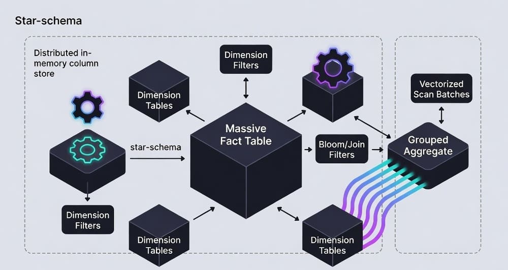
Star transformation (a.k.a. star join optimization)

BI queries over a star schema: big FACT_SALES with multiple small DIM_* tables.
The optimizer:
1. Filters each dimension (pushdown predicates).
2. Builds join filters (often Bloom filters or bitmaps).
3. Semi-joins the fact to prune row groups before full join/aggregate.
Result: the fact scan skips vast swaths; you aggregate far less data.

In-memory vs. “in-cache”

True in-memory column store keeps working sets resident and executes vector ops from RAM/CPU cache.
Many cloud warehouses rely on aggressive caching + SSD spill. That’s fine—until concurrency spikes or a cold start.

A concrete example (Snowflake & DuckDB flavored)

Schema (shortened):

-- Fact table (billions of rows)
CREATE TABLE FACT_SALES(
  date_id        DATE,
  store_id       INT,
  product_id     INT,
  qty            INT,
  gross_amount   NUMBER(12,2),
  net_amount     NUMBER(12,2)
);

-- Dimensions (small)
CREATE TABLE DIM_DATE(..., is_weekend BOOLEAN, fiscal_qtr STRING);
CREATE TABLE DIM_STORE(store_id INT, region STRING, country STRING);
CREATE TABLE DIM_PRODUCT(product_id INT, category STRING, brand STRING);

Query pattern (star transformation target):

-- BI query: last 8 quarters, only "Beverage" and selected regions
SELECT  d.fiscal_qtr,
        p.category,
        SUM(f.net_amount) AS revenue,
        SUM(f.qty)        AS units
FROM FACT_SALES f
JOIN DIM_DATE    d ON f.date_id    = d.date_id
JOIN DIM_PRODUCT p ON f.product_id = p.product_id
JOIN DIM_STORE   s ON f.store_id   = s.store_id
WHERE d.fiscal_qtr BETWEEN 'FY23Q1' AND 'FY24Q4'
  AND p.category = 'Beverage'
  AND s.region IN ('NE','SE')
GROUP BY d.fiscal_qtr, p.category;

What a smart engine does under the hood

Filters DIM_DATE, DIM_PRODUCT, DIM_STORE.
Builds Bloom filters for product_id and store_id.
Applies filters during the vectorized fact scan, discarding row groups early.
Aggregates vectors with SIMD (sum/min/max/count are extremely fast on compressed, typed vectors).

DuckDB / local vectorized demo sketch (Python)

import duckdb
con = duckdb.connect()
# Assume parquet files partitioned by date
con.execute("""
SELECT d.fiscal_qtr, p.category, SUM(f.net_amount) AS revenue
FROM 's3://bucket/fact_sales/*.parquet' f
JOIN dim_product p USING(product_id)
JOIN dim_date d USING(date_id)
WHERE d.fiscal_qtr BETWEEN 'FY23Q1' AND 'FY24Q4'
  AND p.category='Beverage'
GROUP BY d.fiscal_qtr, p.category;
""")

DuckDB automatically vectorizes; on large Parquet it will prune columns and partitions, then push filters into the scan.

Cost/Benefit: Do you really need more RAM?

Back-of-envelope sizing (pragmatic, not vendor hype)

Let:

C = Compressed size of the columns actually scanned for hot dashboards.
α = Expansion factor during execution (decompression + vectors + hash tables). Typical 1.3–3.0×.
K = Peak concurrency (simultaneous heavy dashboards).
S = Safety margin (~1.2× to absorb bursts).

Then required RAM for “fully in-memory hot set”:

RAM ≈ C × α × K × S

Example

You scan 4 columns of FACT_SALES compressed to 250 GB total for top BI queries.
α = 2.0, K = 6, S = 1.25 → RAM ≈ 250 × 2 × 6 × 1.25 = 3.75 TB.
If you only keep the 90-day hot window in memory (say 60 GB compressed), RAM drops to ~900 GB with same assumptions.

When RAM is worth it

Repeated, latency-sensitive dashboards (sub-second expectations).
High selectivity predicates on dimensions (star transformation pays off).
Heavy group-bys on a few numeric columns (vector aggregates scream).

When to save your budget

Ad-hoc, scan-everything exploration on wide tables—SSD + compressed columnar often suffices.
If predicates are unselective (you scan most of the fact anyway).
If concurrency is modest and caches stay warm.

Comparison table (what actually changes)

Technique	What it does	Wins	Trade-offs	Best for
Row store + nested loops	Row-at-a-time execution	Simple	CPU overhead, cache misses	OLTP
Column store (disk)	Column pruning + compression	Large I/O savings	Cold-start I/O	General BI
Vectorized scans	SIMD on column batches	CPU efficiency	Requires batch-friendly ops	Aggregations, filters
Star transformation	Prune fact by dim filters	Massive data skipping	Needs good stats & keys	Star-schema BI
In-memory column store	Keep hot set in RAM	Sub-second UX, concurrency	RAM cost, eviction strategy	High-traffic dashboards

Best practices (and common faceplants)

Modeling

Keep dimensions small & selective. High-cardinality dims still work, but avoid bloat.
Surrogate keys and uniform distributions help join filters.
Partition facts by time, cluster by frequent filters (e.g., store_id, product_id).

Storage & files

Parquet/ORC with row groups ~128–512 MB; avoid millions of tiny files.
Use zstd or lz4; prefer codecs that keep data vector-friendly.

Stats & pruning

Maintain statistics so the optimizer dares to star-transform.
Enable features like dynamic data pruning / join filtering.

Execution

Aim for narrow scans: project only needed columns.
Watch vector size and spill thresholds; small vectors kill SIMD wins.

Concurrency & caching

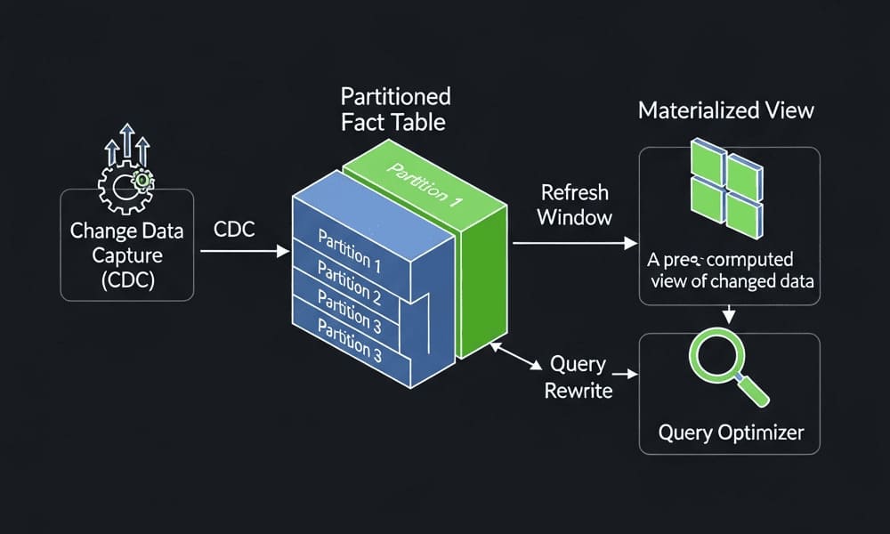
Separate hot vs. cold data. Keep a 90–180 day window hot; age out the rest.
Use result cache/materialized views for top tiles; refresh incrementally.

Anti-patterns

“Throw RAM at it” without measuring C, α, K.
Joining on non-selective dimensions and expecting miracles.
Over-indexing a column store like it’s a row store.

Conclusion & takeaways

Speed ≠ RAM alone. You need columnar compression, vectorized operators, and star transformations working together.
Size the hot set, not the lake. Keep the 90–180 day BI window in memory; let the rest live on disk/SSD.
Measure, then buy. Calculate C × α × K × S before ordering more memory.

If your dashboards still stutter: your dimensions aren’t selective, your files are too small, or your engine isn’t truly vectorized. Fix those before you open the wallet.

Internal link ideas

Star Schema vs. Single-Table Design for Analytics
How Vectorized Execution Works (SIMD, cache lines, batch size)
Data Skipping 101: Min/Max, Zone Maps, and Bloom Filters
Materialized Views for BI: Freshness vs. Cost
DuckDB vs. ClickHouse vs. Snowflake for Interactive BI

Image prompt

“A clean, modern data architecture diagram of a star-schema on a distributed in-memory column store. Show dimension filters generating Bloom/join filters that prune a massive fact table. Emphasize vectorized scan batches flowing through to a grouped aggregate. Minimalist, high contrast, isometric 3D style.”

Data/ML Engineer Blog