The common Doris performance problem is a handful of BI queries that join a few large tables all day. Broadcast is too big, full shuffle is too slow, and the dashboard still needs sub-second metrics. Doris can make those joins effectively local so the network stops being the bottleneck - the two strategies that do it are Colocation Join and Bucket Shuffle Join. Used correctly they make dashboards feel instant; used wrong, you're back to shuffling mountains of data across the cluster.
Four ways Doris moves data for joins
| Method | Network cost | When it applies |
|---|---|---|
| Broadcast | N × T(R) | Small right side, many join nodes |
| Partition Shuffle | T(S) + T(R) | General hash joins |
| Bucket Shuffle | T(R) | Join key hits the left table's bucket column; left is a single partition |
| Colocation | ≈ 0 | Both sides already hash-distributed identically, in the same colocate group |
As the distribution requirements get stricter, performance generally improves - but with one trap: too few buckets reduces parallelism and can make Bucket Shuffle or Colocation slower than an ordinary shuffle.
What each strategy means
Bucket Shuffle is the fast, flexible one. When the join condition includes the left table's bucket column, Doris keeps the left table in place and moves only the right side to the matching buckets - which is why the cost is T(R) instead of T(S)+T(R). The planner chooses it automatically when the conditions hold: an equality join, bucket columns on both sides, and (for physical tables) a single-partition left side to guarantee correctness.
Colocation is the fastest and the strictest. If both tables are already hash-distributed on the same keys with the same bucket count and replica count, Doris joins locally with no shuffle at all. You enforce it by placing tables in the same colocation group via PROPERTIES("colocate_with"="..."). If the group becomes unstable - during replica repair or rebalancing - Doris degrades to a normal shuffle plan until it stabilizes again.
Enforcing Colocation
CREATE TABLE fact_orders (
  dt DATE, user_id BIGINT, sku BIGINT, qty INT, price BIGINT
)
DUPLICATE KEY(dt, user_id)
PARTITION BY RANGE(dt) (PARTITION p2025_11 VALUES LESS THAN ("2025-12-01"))
DISTRIBUTED BY HASH(user_id) BUCKETS 32
PROPERTIES ("replication_num" = "3", "colocate_with" = "sales_cg");

CREATE TABLE dim_users (
  user_id BIGINT, city VARCHAR(64), segment VARCHAR(32)
)
DUPLICATE KEY(user_id)
DISTRIBUTED BY HASH(user_id) BUCKETS 32          -- must match: key, buckets, replicas
PROPERTIES ("replication_num" = "3", "colocate_with" = "sales_cg");
Verify the plan is local - a colocated plan's EXPLAIN string includes colocate: true; if the group is unstable you'll see it fall back to a broadcast or shuffle:
EXPLAIN SELECT 1 FROM fact_orders f JOIN dim_users d ON f.user_id = d.user_id;

SHOW PROC '/colocation_group';   -- admin: check IsStable=true; joins degrade while false
Tables can move in and out of a group later, and replication for a colocate group is changed at the group level so the members stay aligned:
ALTER TABLE fact_orders SET ("colocate_with" = "sales_cg");   -- add / move
ALTER TABLE fact_orders SET ("colocate_with" = "");           -- remove
ALTER COLOCATE GROUP sales_cg SET ("replication_num" = "3");  -- group-level replicas
For cross-database joins, use a global group with the __global__ prefix in colocate_with.
Nudging the planner toward Bucket Shuffle
Bucket Shuffle is about query shape more than DDL. Keep the left side on its bucket distribution and prune it to a single partition so the planner can use it:
EXPLAIN
SELECT SUM(f.qty * f.price) AS revenue, d.segment
FROM fact_orders f
JOIN dim_users d ON f.user_id = d.user_id   -- join uses the left bucket column
WHERE f.dt = '2025-11-15'                    -- single partition on the left
GROUP BY d.segment;
A fitting plan shows join op: ... (BUCKET_SHUFFLE) with the right side exchanged to the left. If the constraints can't be met, Doris falls back to partition shuffle. There is no explicit bucket-shuffle hint - Doris selects it automatically - but you can force the right table's distribution with [shuffle] or [broadcast] hints when colocation isn't possible and the planner didn't pick what you want:
SELECT COUNT(*) FROM big_left l JOIN [broadcast] small_dim r ON r.k = l.k;Choosing between them
Use Colocation when the same keys drive most joins (e.g. user_id or order_id), you control the table design and can align keys, bucket count, and replication, and you need the lowest latency and can live with the stricter layout - it gives true zero-shuffle local joins while the group is stable. Use Bucket Shuffle when joins vary or only one side is aligned, and you can filter the left to a single partition with the join column as the left's bucket column - it moves only the right side and is far easier to satisfy than full colocation.
Common pitfalls
- Group "unstable," plan shuffles anyway. Normal during balancing or repair - wait for stability, or pause auto-balance temporarily if it's hurting SLAs.
- Mismatched bucket counts or replica numbers. You won't get colocated joins until these match across the group.
- Left table isn't single-partition. Bucket Shuffle may not trigger - add a date filter or refactor partitions.
- Too few buckets. You've killed parallelism; increase buckets and rebalance.
End-to-end example
-- Two tables aligned for colocation
CREATE TABLE a (k BIGINT, v BIGINT) DISTRIBUTED BY HASH(k) BUCKETS 16
PROPERTIES("replication_num"="3", "colocate_with"="cg_demo");
CREATE TABLE b (k BIGINT, v BIGINT) DISTRIBUTED BY HASH(k) BUCKETS 16
PROPERTIES("replication_num"="3", "colocate_with"="cg_demo");

SHOW PROC '/colocation_group';                         -- verify group status
EXPLAIN SELECT SUM(a.v+b.v) FROM a JOIN b USING(k);    -- expect colocate: true

-- Bucket Shuffle pattern (left pruned to one partition)
EXPLAIN
SELECT COUNT(*)
FROM fact_orders f                 -- partitioned by dt, bucketed by user_id
JOIN dim_users d ON f.user_id = d.user_id
WHERE f.dt = CURRENT_DATE();       -- prune to one partition on the left
The short version
Colocation gives the best latency under a strict layout - same keys, buckets, replicas, and a stable group. Bucket Shuffle gives nearly as good latency under looser constraints - the left's bucket column in the join and a single-partition left. In both cases, verify the chosen plan with EXPLAIN and keep an eye on group stability, because a degraded group quietly loses the colocated plan. A good way to start: take your two most expensive joins, give one a colocate group and shape the other's SQL to hit Bucket Shuffle, and measure the plan and latency before and after.

Leave a Comment