Designing for Semi-Structured Data in Snowflake: VARIANT, Nested JSON, and Search Optimization Service
Hook: Your product logs, clickstream events, and API payloads rarely agree on a schema—and they change weekly. You can either fight that chaos with fragile ETL, or design for it. This guide shows how to model and query semi-structured data in Snowflake using VARIANT, nested JSON, and Search Optimization Service (SOS)—with clear patterns, performance tactics, and trade-offs.
Why this matters
- Semi-structured formats (JSON/Parquet/Avro) evolve fast; rigid tables don’t.
VARIANTlets you land anything quickly, while still letting you prune scans, index hot paths, and materialize stable fields.- Done right, you keep ingestion simple and queries fast. Done wrong, you pay in scans, flatten explosions, and unpredictable costs.
Core concepts & architecture
Landing pattern (schema-on-ingest, structure-on-demand)
- Land raw events/files into a table with a
VARIANTcolumn (payload). - Project commonly-used fields into typed columns (computed or materialized).
- Accelerate selective lookups with Search Optimization on key JSON paths.
- Materialize heavy joins/aggregations via views, dynamic tables, or MVs.
Raw Stage (S3/GCS/Azure) --> RAW_EVENTS(payload VARIANT)
                                  |
                                  v
             Derived Columns / Projections (views or dynamic tables)
                                  |
                                  v
                BI/ML/Apps with fast, typed access + SOS on hot paths
When to use VARIANT vs typed columns
| Scenario | Use VARIANT | Use Typed Columns |
|---|---|---|
| Highly evolving schema | ✅ | ❌ |
| A few hot fields queried constantly | ➖ keep raw + project hot fields | ✅ for hot fields |
| Strict type enforcement needed | ❌ | ✅ |
| Rare forensic/debug queries | ✅ | ❌ |
| Heavy joins/aggregations | ➖ start raw, then materialize | ✅ |
Modeling patterns that work
1) Envelope pattern for events
Keep a consistent wrapper even if the body changes.
create table raw_events (
  event_time  timestamp_ntz,
  event_name  string,
  source      string,
  payload     variant -- nested JSON
);

-- Ingest
copy into raw_events
from @my_stage
file_format=(type=json strip_outer_array=true);
2) Project hot paths (computed columns)
Expose frequently filtered or joined fields as typed, not only as JSON paths.
create or replace table raw_events_projected as
select
  event_time,
  event_name,
  source,
  payload,
  -- projections
  payload:"user".id::string        as user_id,
  payload:"order".id::string       as order_id,
  payload:"order".total::number    as order_total,
  payload:"geo".country::string    as country
from raw_events;
Benefits:
- Type checking early.
- Micro-partition pruning works better with native columns.
- Simpler joins and aggregations.
3) Late-binding for “maybe” fields
Use COALESCE across alternative locations to normalize drift:
select
  coalesce(payload:"user".id::string, payload:"actor".id::string) as user_id_norm
from raw_events;
4) Controlled flattening
Flatten only when needed and keep scope tight to avoid row explosions.
select
  event_time,
  event_name,
  i.value::string as item_id
from raw_events,
lateral flatten(input => payload:"items", outer => false) i
where event_name = 'checkout';
Tips
- Filter before flatten where possible (on outer fields).
- Avoid recursive flatten unless truly required.
Query performance fundamentals
Micro-partition pruning with JSON
Snowflake can prune using JSON path predicates if you filter with sargable conditions:
-- Good: sargable (enables pruning)
where payload:"geo".country::string = 'DE'

-- Risky: wrapping the path in functions can block pruning
where lower(payload:"geo".country::string) = 'de'
Rule of thumb: Put simple equality/range predicates directly on the path or its cast; avoid wrapping in non-sargable functions on the left side.
Cluster keys (use sparingly)
If most queries filter on a single projected column (e.g., event_time, user_id), clustering can improve pruning:
alter table raw_events_projected cluster by (event_time);
Don’t over-cluster; maintenance has costs. Start with time, then consider 1–2 additional high-selectivity columns.
Search Optimization Service (SOS): when and how
What it is: A Snowflake service that builds an auxiliary search access path to speed up selective lookups on columns or JSON paths—especially useful when micro-partition pruning isn’t enough.
Great for
WHERE payload:"order".id::string = 'o_123'EXISTSchecks within arrays, nested attributes with high selectivity- Ad-hoc investigative queries on sparse fields
Not great for
- Low-selectivity predicates (e.g.,
country IN ('US','CA')) - Full scans/aggregations where pruning dominates anyway
- Rapidly changing wide tables without clear lookup patterns
Creating SOS on JSON paths
Narrow the scope to hot, selective paths to control cost:
-- Add SOS on two JSON paths and one typed column
create or replace search optimization on raw_events_projected
  on (payload:"order".id::string, payload:"user".id::string, user_id);
You can also target arrays and nested structures:
create or replace search optimization on raw_events
  on (payload:"items"[*].sku::string);
Operational tips
- Monitor query plans: ensure the “Search optimization” access path appears where expected.
- Revisit paths quarterly; drop unused ones.
- Prefer creating SOS after projecting the field as a column if you query it constantly.
A realistic example end-to-end
1) Raw table with JSON
create or replace table raw_events (
  event_time timestamp_ntz,
  event_name string,
  payload    variant
);
2) Projections + light normalization (view)
create or replace view v_events as
select
  event_time,
  event_name,
  payload,
  payload:"user".id::string               as user_id,
  coalesce(payload:"order".id::string, payload:"purchase".id::string) as order_id,
  payload:"order".total::number           as order_total,
  payload:"geo".country::string           as country
from raw_events;
3) Search optimization on hot lookups
create or replace search optimization on v_events
  on (user_id, order_id);
4) Fast “needle in a haystack” queries
-- Look up a single order quickly
select * from v_events
where order_id = 'o_9012' and event_time >= dateadd(day,-7,current_date);

-- Investigate a user's funnel
select event_time, event_name
from v_events
where user_id = 'u_42'
order by event_time;
5) Materialize for BI (optional, for heavy workloads)
Use dynamic tables to maintain a typed, join-friendly shape:
create or replace dynamic table dt_orders
target_lag = '5 minutes'
as
select
  order_id,
  max_by(order_total, event_time) as latest_order_total,
  count_if(event_name = 'checkout') as checkout_events_7d
from v_events
where event_time >= dateadd(day, -30, current_date)
group by order_id;

-- Consider SOS on order_id if investigative lookups remain common
Best practices & common pitfalls
Best practices
- Project the top 5–10 fields you filter/join on. Keep the rest in
payload. - Keep predicates sargable: simple comparisons on casts (no unnecessary functions).
- Flatten surgically: only the array you need, and only after outer filters.
- SOS with intent: index only selective paths with clear business questions.
- Version payloads: include a
schema_versionorevent_versioninside JSON to track evolution. - Guardrails: create views with whitelisted fields for analysts to avoid accidental deep nesting scans.
Pitfalls
- Function-wrapped filters on JSON paths → kills pruning.
- Over-flattening → row explosion, surprise costs.
- Indexing everything with SOS → unnecessary spend; keep it narrow.
- Skipping projections and forcing every query through JSON → slower joins/aggregations.
- Assuming SOS helps aggregates → it’s for lookups, not for wide scans.
Conclusion & takeaways
- Use
VARIANTto land fast and survive schema drift. - Project the hot fields to typed columns for joins and pruning.
- Use Search Optimization to supercharge selective lookups on JSON paths.
- Materialize heavy transforms via dynamic tables or materialized views.
- Keep filters sargable, flatten carefully, and index only what matters.
Next steps: pick one workload (e.g., order investigations), project the 5 key fields, add a minimal SOS on those paths, and measure the before/after query profile.
Internal link ideas
- Sharding Strategies 101: Range vs Hash vs Directory
- Real-Time Analytics on NoSQL + Snowflake: Streams & Materialized Views
- DynamoDB Single-Table vs Snowflake: Designing Access Patterns
- JSON UDFs and Performance: When to Move Logic to SQL
Image prompt
“A clean, modern data architecture diagram showing a Snowflake table with a VARIANT JSON column, projections to typed columns, a focused Search Optimization index on hot JSON paths, and a downstream dynamic table for BI — minimalistic, high contrast, 3D isometric style.”
Tags
#Snowflake #VARIANT #JSON #SearchOptimization #DataEngineering #Performance #Modeling #SemiStructured #SQL #Architecture


Leave a Reply